
반응형
Notice
Recent Posts
Recent Comments
Link
| 일 | 월 | 화 | 수 | 목 | 금 | 토 |
|---|---|---|---|---|---|---|
| 1 | 2 | 3 | ||||
| 4 | 5 | 6 | 7 | 8 | 9 | 10 |
| 11 | 12 | 13 | 14 | 15 | 16 | 17 |
| 18 | 19 | 20 | 21 | 22 | 23 | 24 |
| 25 | 26 | 27 | 28 | 29 | 30 | 31 |
Tags
- 프롬프트 커스터마이징
- MNIST
- AutoGPT
- 특징 교차
- 차원의 저주
- .perfcc
- ubuntu
- 비선형변환
- GPT4
- 하둡
- hadoop
- .mongorc.js
- MYSQL
- perfcc
- 생성다항식
- 셸 작업
- python
- centos7
- Power BI
- 스크립트
- PCA
- 셸 소개
- 도큐먼트
- AWS
- 머신러닝
- Retention
- 스머프 공격
- DDL
- SQL
- Tableau
Archives
- Today
- Total
데이터의 민족
< 핸즈온 머신러닝 - 모델훈련 > 본문
728x90
반응형
SMALL
Chapter_4 모델 훈련.ipynb
Colaboratory notebook
colab.research.google.com
1. 선형 회귀
- 입력 특성의 가중치 합과 편향이라는 상수를 더해 예측을 만듦
- 선형 회귀 모델을 훈련시키려면 RMSE, MSE를 최소화하는 파라미터를 찾아야함
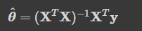
1 - 1. 정규방정식
- 비용 함수를 최소화하는 파라미터값을 찾기 위한 해석적인 방법, 수학 공식을 의미
import numpy as np
import pandas as pd
import matplotlib.pyplot as plt

X = 2 * np.random.rand(100, 1)
y = 4 + 3 * X + np.random.randn(100, 1)

plt.plot(X, y, "b.")
plt.xlabel("$x_1$", fontsize=18)
plt.ylabel("$y$", rotation=0, fontsize=18)
plt.axis([0, 2, 0, 15])
plt.show()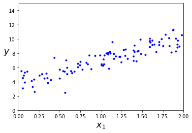
- 넘파이 선형대수 모듈(np.linalg)에 있는 inv()함수를 사용해 역행렬 계산
- dot() 메서드를 사용해 행렬 곱셈
X_b = np.c_[np.ones((100, 1)), X]  # 모든 샘플에 x0 = 1을 추가합니다.
theta_best = np.linalg.inv(X_b.T.dot(X_b)).dot(X_b.T).dot(y)

theta_best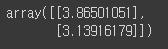
- 예측
X_new = np.array([[0], [2]])
X_new_b = np.c_[np.ones((2, 1)), X_new]  # 모든 샘플에 x0 = 1을 추가합니다.
y_predict = X_new_b.dot(theta_best)
y_predict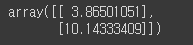
- 시각화
plt.plot(X_new, y_predict, "r-")
plt.plot(X, y, "b.")
plt.axis([0, 2, 0, 15])
plt.show()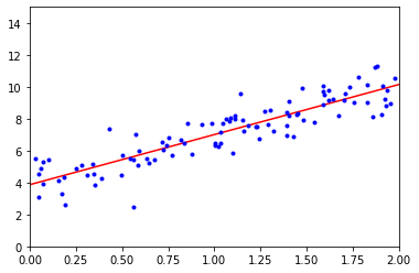
1 - 2. 사이킷런에서 선형 회귀 수행
from sklearn.linear_model import LinearRegression

lin_reg = LinearRegression()
lin_reg.fit(X, y)
lin_reg.intercept_, lin_reg.coef_
lin_reg.predict(X_new)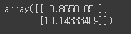
- LinearRegression 클래스는 scipy.linalg.lstsq()함수(최소 제곱)를 기반
- 이 함수는 X+y을 계산합니다. X+는 X의 유사역행렬(pseudoinverse)
- 정확하게는 Moore–Penrose 유사역행렬
- np.linalg.pinv()을 사용해서 유사역행렬을 직접 계산
- 유사역행렬 자체는 특잇값 분해(SVD)라 부르는 표준 행렬 분해 기법을 사용해 계산
- np.linalg.svd()
# 싸이파이 lstsq() 함수를 사용하려면 scipy.linalg.lstsq(X_b, y)와 같이 씁니다.
theta_best_svd, residuals, rank, s = np.linalg.lstsq(X_b, y, rcond=1e-6)
theta_best_svd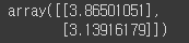
1 - 3. 계산 복잡도
- 역행렬을 계산
- 일반적으로 O(n ** 2.4)에서 O(n*n*n) 사이
- 예측 계산 복잡도는 샘플 수와 특성 수에 선형적
2. 경사 하강법
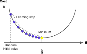
- 여러 종류의 문제에서 최적의 해법을 찾을 수 있는 일반적인 최적화 알고리즘
- 비용 함수를 최소화하기 위해서 반복해서 파라미터를 조정
- 파라미터를 임의의 값으로 시작해서(무작위 초기화) 한 번에 조금씩 비용 함수가 감소되는 방향으로 진행
- 알고리즘이 최솟값에 수렴할 때까지 점진적으로 향상
- 중요한 파라미터는 스텝의 크기로, 학습률 하이퍼파라미터로 결정
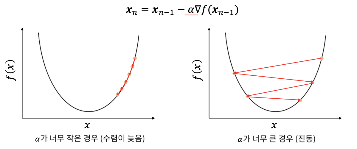
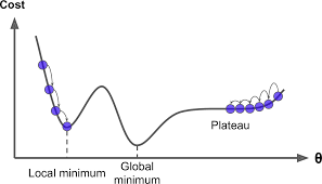
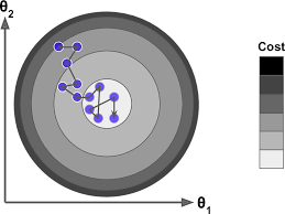
- 경사 하강법의 문제점
- Local minimum: 지역 최솟값
- Global minimum: 전역 최솟값
- Plateau: 평지
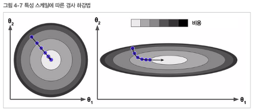
- 왼쪽: 특정 스케일 적용 /오른쪽: 특정 스케일 적용 안함
2 - 1. 배치 경사 하강법
- 편도 함수: 파라미터가 조금 변경될 때 비용 함수가 얼마나 바뀌는지 계산
- 비용 함수의 편도 함수
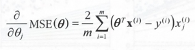
- 비용 함수의 그레디언트 벡터
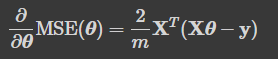
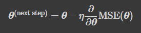
- 경사 하강법의 스텝
eta = 0.1  # 학습률
n_iterations = 1000
m = 100

theta = np.random.randn(2,1)  # 랜덤 초기화

for iteration in range(n_iterations):
    gradients = 2/m * X_b.T.dot(X_b.dot(theta) - y)
    theta = theta - eta * gradients

theta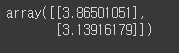
- 세 가지의 다른 학습률을 사용하여 진행한 경사 하강법의 스템 처음 10개 시각화(점선 부분이 시작)
theta_path_bgd = []

def plot_gradient_descent(theta, eta, theta_path=None):
    m = len(X_b)
    plt.plot(X, y, "b.")
    n_iterations = 1000
    for iteration in range(n_iterations):
        if iteration < 10:
            y_predict = X_new_b.dot(theta)
            style = "b-" if iteration > 0 else "r--"
            plt.plot(X_new, y_predict, style)
        gradients = 2/m * X_b.T.dot(X_b.dot(theta) - y)
        theta = theta - eta * gradients
        if theta_path is not None:
            theta_path.append(theta)
    plt.xlabel("$x_1$", fontsize=18)
    plt.axis([0, 2, 0, 15])
    plt.title(r"$\eta = {}$".format(eta), fontsize=16)


np.random.seed(42)
theta = np.random.randn(2,1)  # random initialization

plt.figure(figsize=(10,4))
plt.subplot(131); plot_gradient_descent(theta, eta=0.02)
plt.ylabel("$y$", rotation=0, fontsize=18)
plt.subplot(132); plot_gradient_descent(theta, eta=0.1, theta_path=theta_path_bgd)
plt.subplot(133); plot_gradient_descent(theta, eta=0.5)

plt.show()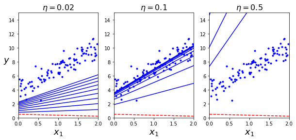
- 왼쪽: 학습률이 너무 낮음, 알고리즘은 최적점에 도착하지만 시간이 오래 걸림
- 가운데: 학습률 적당, 반복 몇 번 만에 이미 최적점 수렴
- 오른쪽: 학습률이 너무 높음, 스템마다 최적점에서 멀어짐
2 - 2. 확률적 경사 하강법
- 배치 경사 하강법의 가장 큰 문제는 매 스텝에서 전체 훈련 세트를 사용해 그레이디언트를 계산
- 훈련 세트가 커지면 매우 느려짐
- 정의: 확률적 경사 하강법은 매 스텝에서 한 개의 샘플을 무작위로 선택, 그 하나의 샘플의 그레이디언트를 계산
- 그러나 무작위 선택으로 배치 경사 하강법보다 불안
- 비용함수 최솟값에 다다를 때까지 요동치며 평균적으로 감소 -> 최솟값에 안착 불가
- 무작위성: 최솟값에서 탈출시켜줘서 좋지만, 알고리즘을 전역 최솟값에 다다르지 못한다는 한계
- 해결방법: 학습률을 점진적으로 감소
- 시작할때 학습률을 크게 하고, 점차적으로 학습률을 감소(너무 빠르지도, 너무 천천히도 안됨)
theta_path_sgd = []
m = len(X_b)
np.random.seed(42)

n_epochs = 50
t0, t1 = 5, 50  # 학습 스케줄 하이퍼파라미터

def learning_schedule(t):
    return t0 / (t + t1)

theta = np.random.randn(2,1)  # 랜덤 초기화

for epoch in range(n_epochs):
    for i in range(m):
        if epoch == 0 and i < 20:
            y_predict = X_new_b.dot(theta)
            style = "b-" if i > 0 else "r--"
            plt.plot(X_new, y_predict, style)
        random_index = np.random.randint(m)
        xi = X_b[random_index:random_index+1]
        yi = y[random_index:random_index+1]
        gradients = 2 * xi.T.dot(xi.dot(theta) - yi)
        eta = learning_schedule(epoch * m + i)
        theta = theta - eta * gradients
        theta_path_sgd.append(theta)

plt.plot(X, y, "b.")
plt.xlabel("$x_1$", fontsize=18)
plt.ylabel("$y$", rotation=0, fontsize=18)
plt.axis([0, 2, 0, 15])
plt.show()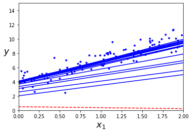
- 사이킷런에서 SGD방식으로 선형회귀를 사용하려면 기본값으로 제곱 오차 비용 함수를 최적화하는 SGDRgressor 클래스 사용
from sklearn.linear_model import SGDRegressor

sgd_reg = SGDRegressor(max_iter=1000, tol=1e-3, penalty=None, eta0=0.1, random_state=42)
sgd_reg.fit(X, y.ravel())

sgd_reg.intercept_, sgd_reg.coef_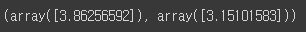
2 - 3. 미니배치 경사 하강법
- 미니배치라 부르는 임의의 작은 샘플 세트에 대해 그레이디언트를 계산
- 행렬 연산에 최적화된 하드웨어, 특히 GPU를 사용해 얻는 성능 향상
- SGD보다 덜 불규칙하게 움직여서 최솟값에 더 가까이 도달
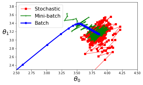
- 세 가지 경사 하강법 알고리즘의 훈련과정 동안 파라미터가 공간에서 움직인 경로
theta_path_mgd = []

n_iterations = 50
minibatch_size = 20

np.random.seed(42)
theta = np.random.randn(2,1)  # 랜덤 초기화

t0, t1 = 200, 1000
def learning_schedule(t):
    return t0 / (t + t1)

t = 0
for epoch in range(n_iterations):
    shuffled_indices = np.random.permutation(m)
    X_b_shuffled = X_b[shuffled_indices]
    y_shuffled = y[shuffled_indices]
    for i in range(0, m, minibatch_size):
        t += 1
        xi = X_b_shuffled[i:i+minibatch_size]
        yi = y_shuffled[i:i+minibatch_size]
        gradients = 2/minibatch_size * xi.T.dot(xi.dot(theta) - yi)
        eta = learning_schedule(t)
        theta = theta - eta * gradients
        theta_path_mgd.append(theta)
theta_path_bgd = np.array(theta_path_bgd)
theta_path_sgd = np.array(theta_path_sgd)
theta_path_mgd = np.array(theta_path_mgd)
plt.figure(figsize=(7,4))
plt.plot(theta_path_sgd[:, 0], theta_path_sgd[:, 1], "r-s", linewidth=1, label="Stochastic")
plt.plot(theta_path_mgd[:, 0], theta_path_mgd[:, 1], "g-+", linewidth=2, label="Mini-batch")
plt.plot(theta_path_bgd[:, 0], theta_path_bgd[:, 1], "b-o", linewidth=3, label="Batch")
plt.legend(loc="upper left", fontsize=16)
plt.xlabel(r"$\theta_0$", fontsize=20)
plt.ylabel(r"$\theta_1$ ", fontsize=20, rotation=0)
plt.axis([2.5, 4.5, 2.3, 3.9])
plt.show()- 빨: 확률적
- 초: 미니배치
- 파: 배치
3. 다항 회귀
- 각 특성의 거듭제곱을 새로운 특성으로 추가하고, 이 확장된 특성을 포함한 데이터 셋에 선형 모델을 훈련
import numpy as np
import numpy.random as rnd

np.random.seed(42)

m = 100
X = 6 * np.random.rand(m, 1) - 3
y = 0.5 * X**2 + X + 2 + np.random.randn(m, 1)

plt.plot(X, y, "b.")
plt.xlabel("$x_1$", fontsize=18)
plt.ylabel("$y$", rotation=0, fontsize=18)
plt.axis([-3, 3, 0, 10])

plt.show()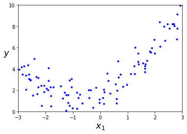
- 사이킷런의 PolynomialFeatures를 사용해 훈련 데이터 변환
- PolynomialFeatures(degree=d)는 특성이 n개인 배열의 특성이 (n+d)! / d!n! 개인 배열로 변환
from sklearn.preprocessing import PolynomialFeatures
poly_features = PolynomialFeatures(degree=2, include_bias=False)
X_poly = poly_features.fit_transform(X)

print(X[0])
print(X_poly[0])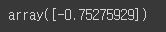
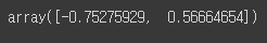
- X_poly는 원래 특성 X와 이 특성의 제곱을 포함
- 확장된 훈련 데이터에 LinearRegression 적용
X_new=np.linspace(-3, 3, 100).reshape(100, 1)
X_new_poly = poly_features.transform(X_new)
y_new = lin_reg.predict(X_new_poly)
plt.plot(X, y, "b.")
plt.plot(X_new, y_new, "r-", linewidth=2, label="Predictions")
plt.xlabel("$x_1$", fontsize=18)
plt.ylabel("$y$", rotation=0, fontsize=18)
plt.legend(loc="upper left", fontsize=14)
plt.axis([-3, 3, 0, 10])

plt.show()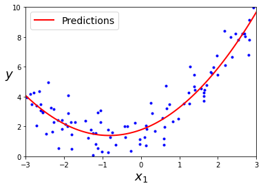
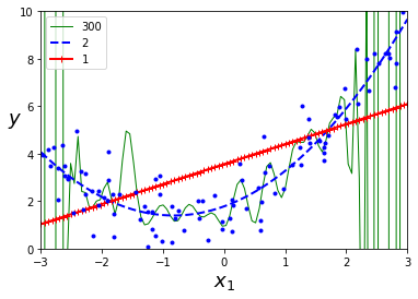
4. 학습 곡선
from sklearn.preprocessing import StandardScaler
from sklearn.pipeline import Pipeline

for style, width, degree in (("g-", 1, 300), ("b--", 2, 2), ("r-+", 2, 1)):
    polybig_features = PolynomialFeatures(degree=degree, include_bias=False)
    std_scaler = StandardScaler()
    lin_reg = LinearRegression()
    polynomial_regression = Pipeline([
            ("poly_features", polybig_features),
            ("std_scaler", std_scaler),
            ("lin_reg", lin_reg),
        ])
    polynomial_regression.fit(X, y)
    y_newbig = polynomial_regression.predict(X_new)
    plt.plot(X_new, y_newbig, style, label=str(degree), linewidth=width)

plt.plot(X, y, "b.", linewidth=3)
plt.legend(loc="upper left")
plt.xlabel("$x_1$", fontsize=18)
plt.ylabel("$y$", rotation=0, fontsize=18)
plt.axis([-3, 3, 0, 10])

plt.show()- 아래 그림의 고차 다항 회귀 모델은 심각하게 훈련 데이터에 과대적합 / 반면에 선형 모델은 과소적합
- 학습 곡선은 일반화 성능 추정의 다른 방법 중 하나
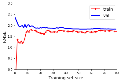
- 단순 선형 회귀 모델의 학습 곡선
from sklearn.metrics import mean_squared_error
from sklearn.model_selection import train_test_split

def plot_learning_curves(model, X, y):
    X_train, X_val, y_train, y_val = train_test_split(X, y, test_size=0.2, random_state=10)
    train_errors, val_errors = [], []
    for m in range(1, len(X_train) + 1):
        model.fit(X_train[:m], y_train[:m])
        y_train_predict = model.predict(X_train[:m])
        y_val_predict = model.predict(X_val)
        train_errors.append(mean_squared_error(y_train[:m], y_train_predict))
        val_errors.append(mean_squared_error(y_val, y_val_predict))

    plt.plot(np.sqrt(train_errors), "r-+", linewidth=2, label="train")
    plt.plot(np.sqrt(val_errors), "b-", linewidth=3, label="val")
    plt.legend(loc="upper right", fontsize=14)
    plt.xlabel("Training set size", fontsize=14)
    plt.ylabel("RMSE", fontsize=14)

lin_reg = LinearRegression()
plot_learning_curves(lin_reg, X, y)
plt.axis([0, 80, 0, 3])

plt.show()- 그래프가 0에서 시작하므로 훈련 세트에 하나 혹은 두 개의 샘플이 있을 땐 모델이 완벽하게 작동
- 하지만 훈련 세트에 샘플이 추가됨에 따라 잡음도 있고 비선형이기에 완벽한 학습은 불가
- so) 곡선이 어느정도 평편해질 때까지 오차가 계속 상승
- 10차 다항 회귀 모델의 학습 곡선
from sklearn.pipeline import Pipeline

polynomial_regression = Pipeline([
        ("poly_features", PolynomialFeatures(degree=10, include_bias=False)),
        ("lin_reg", LinearRegression()),
    ])

plot_learning_curves(polynomial_regression, X, y)
plt.axis([0, 80, 0, 3])

plt.show()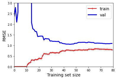
- 두 개의 학습 곡선의 차이점
- 훈련 데이터의 오차가 선형 회귀 모델보다 훨씬 낮음
- 두 곡선 사이에 공간이 존재 / 즉, 훈련 데이터에서의 모델 성능이 검증 데이터에서보다 훨씬 좋음을 의미-> 과대적합 모델의 특징
- 그러나 더 큰 훈련 세트를 사용하면 두 곡선이 점점 가까워짐
- 과대적합 모델을 개선하는 방법: 검증 오차가 훈련 오차에 근접할 때까지 더 많은 훈련 데이터 추가
- 편향 / 분산 트레이드오프: 모델의 일반화 오차는 세 가지 다른 종류의 오차의 합으로 표현
- 편향
- 일반화 오차 중에서 편향은 잘못괸 가정으로 인한 것. 예로, 데이터가 실제로는 2차인데 선형으로 가정하는 경우
- 편향이 큰 모델은 훈련 데이터에 과소적합되기 쉬움
- 분산
- 훈련 데이터에 있는 작은 변동에 모델이 과도하게 민감하기 때문에 나타남
- 자유도가 높은 모델이 높은 분산을 가지기 쉬워 과대적합이 되는 경향
- 줄일 수 없는 오차
- 데이터 자체에 있는 잡음 때문에 발생
- 오차를 줄일 수 있는 유일한 방법은 데이터에서 잡음을 제거하는 것
- 모델의 복잡도가 커지면 -> 분산 증가 / 편향 감소
- 모델의 복잡도가 줄어들면 -> 분산 감소 / 편향 증가
- 편향
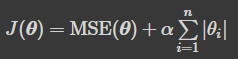
5. 규제가 있는 선형 모델
- 선형 회귀 모델에서 가중치를 제한하는 규제로 릿지, 라쏘, 엘라스틱넷
5 - 1. 릿지
- 학습 알고리즘을 데이터에 맞추는 것뿐만 아니라 모델의 가중치가 가능한 작게 유지되도록 노력
- a = 0이면 릿지 회귀는 선형 회귀와 같아짐
- a가 아주 크면 모든 가중치가 거의 0에 가까워지고 결국 데이터의 평균을 지나는 수평선
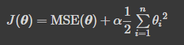
- 편향 는 규제 없음(합 기호가 i = 0이 아니고 i = 1에서 시작)
- W를 특성의 가중치 벡터 (0, 에서 0, )라고 정의하면 규제항은 '(IwIL)'
- 여기서 | 가 가중치 벡터의 , 노름 / 경사 하강법에 적용하려면 MSE 그레이디언트 벡터에 aw를 더하 면 됩니다
- 선형 데이터에 몇 가지의 a를 사용해 릿지 모델 훈련
- 왼쪽: 평범한 릿지
- 오른쪽: PolynomialFeatures(degreee = 10)사용해 먼저 데이터를 확장하고 StandardScaler를 사용
from sklearn.linear_model import Ridge
ridge_reg = Ridge(alpha=1, solver="cholesky", random_state=42)
ridge_reg.fit(X, y)
ridge_reg.predict([[1.5]])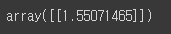
ridge_reg = Ridge(alpha=1, solver="sag", random_state=42)
ridge_reg.fit(X, y)
ridge_reg.predict([[1.5]])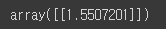
from sklearn.linear_model import Ridge

def plot_model(model_class, polynomial, alphas, **model_kargs):
    for alpha, style in zip(alphas, ("b-", "g--", "r:")):
        model = model_class(alpha, **model_kargs) if alpha > 0 else LinearRegression()
        if polynomial:
            model = Pipeline([
                    ("poly_features", PolynomialFeatures(degree=10, include_bias=False)),
                    ("std_scaler", StandardScaler()),
                    ("regul_reg", model),
                ])
        model.fit(X, y)
        y_new_regul = model.predict(X_new)
        lw = 2 if alpha > 0 else 1
        plt.plot(X_new, y_new_regul, style, linewidth=lw, label=r"$\alpha = {}$".format(alpha))
    plt.plot(X, y, "b.", linewidth=3)
    plt.legend(loc="upper left", fontsize=15)
    plt.xlabel("$x_1$", fontsize=18)
    plt.axis([0, 3, 0, 4])

plt.figure(figsize=(8,4))
plt.subplot(121)
plot_model(Ridge, polynomial=False, alphas=(0, 10, 100), random_state=42)
plt.ylabel("$y$", rotation=0, fontsize=18)
plt.subplot(122)
plot_model(Ridge, polynomial=True, alphas=(0, 10**-5, 1), random_state=42)


plt.show()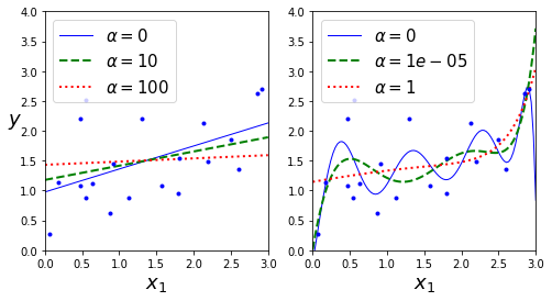
sgd_reg = SGDRegressor(penalty="l2", max_iter=1000, tol=1e-3, random_state=42)
sgd_reg.fit(X, y.ravel())
sgd_reg.predict([[1.5]])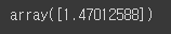
5 - 2. 라쏘
- 릿지 회귀처럼 비용 함수에 규제항을 더함
- 덜 중요한 특성의 가중치를 제거
- 자동으로 특성 선택을 하고 희소 모델을 생성
from sklearn.linear_model import Lasso

plt.figure(figsize=(8,4))
plt.subplot(121)
plot_model(Lasso, polynomial=False, alphas=(0, 0.1, 1), random_state=42)
plt.ylabel("$y$", rotation=0, fontsize=18)
plt.subplot(122)
plot_model(Lasso, polynomial=True, alphas=(0, 10**-7, 1), random_state=42)


plt.show()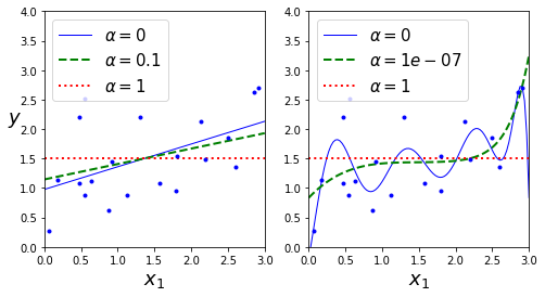
t1a, t1b, t2a, t2b = -1, 3, -1.5, 1.5

t1s = np.linspace(t1a, t1b, 500)
t2s = np.linspace(t2a, t2b, 500)
t1, t2 = np.meshgrid(t1s, t2s)
T = np.c_[t1.ravel(), t2.ravel()]
Xr = np.array([[1, 1], [1, -1], [1, 0.5]])
yr = 2 * Xr[:, :1] + 0.5 * Xr[:, 1:]

J = (1/len(Xr) * np.sum((T.dot(Xr.T) - yr.T)**2, axis=1)).reshape(t1.shape)

N1 = np.linalg.norm(T, ord=1, axis=1).reshape(t1.shape)
N2 = np.linalg.norm(T, ord=2, axis=1).reshape(t1.shape)

t_min_idx = np.unravel_index(np.argmin(J), J.shape)
t1_min, t2_min = t1[t_min_idx], t2[t_min_idx]

t_init = np.array([[0.25], [-1]])
def bgd_path(theta, X, y, l1, l2, core = 1, eta = 0.05, n_iterations = 200):
path = [theta]
for iteration in range(n_iterations):
gradients = core * 2/len(X) * X.T.dot(X.dot(theta) - y) + l1 * np.sign(theta) + l2 * theta
theta = theta - eta * gradients
path.append(theta)
return np.array(path)
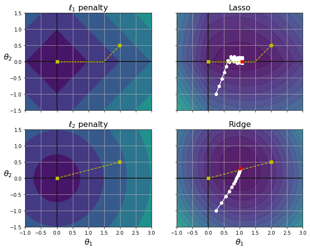
fig, axes = plt.subplots(2, 2, sharex=True, sharey=True, figsize=(10.1, 8))
for i, N, l1, l2, title in ((0, N1, 2., 0, "Lasso"), (1, N2, 0, 2., "Ridge")):
JR = J + l1 * N1 + l2 * 0.5 * N2**2
tr_min_idx = np.unravel_index(np.argmin(JR), JR.shape)
t1r_min, t2r_min = t1[tr_min_idx], t2[tr_min_idx]
levelsJ=(np.exp(np.linspace(0, 1, 20)) - 1) * (np.max(J) - np.min(J)) + np.min(J)
levelsJR=(np.exp(np.linspace(0, 1, 20)) - 1) * (np.max(JR) - np.min(JR)) + np.min(JR)
levelsN=np.linspace(0, np.max(N), 10)
path_J = bgd_path(t_init, Xr, yr, l1=0, l2=0)
path_JR = bgd_path(t_init, Xr, yr, l1, l2)
path_N = bgd_path(np.array([[2.0], [0.5]]), Xr, yr, np.sign(l1)/3, np.sign(l2), core=0)
ax = axes[i, 0]
ax.grid(True)
ax.axhline(y=0, color='k')
ax.axvline(x=0, color='k')
ax.contourf(t1, t2, N / 2., levels=levelsN)
ax.plot(path_N[:, 0], path_N[:, 1], "y--")
ax.plot(0, 0, "ys")
ax.plot(t1_min, t2_min, "ys")
ax.set_title(r"$\ell_{}$ penalty".format(i + 1), fontsize=16)
ax.axis([t1a, t1b, t2a, t2b])
if i == 1:
ax.set_xlabel(r"$\theta_1$", fontsize=16)
ax.set_ylabel(r"$\theta_2$", fontsize=16, rotation=0)
ax = axes[i, 1]
ax.grid(True)
ax.axhline(y=0, color='k')
ax.axvline(x=0, color='k')
ax.contourf(t1, t2, JR, levels=levelsJR, alpha=0.9)
ax.plot(path_JR[:, 0], path_JR[:, 1], "w-o")
ax.plot(path_N[:, 0], path_N[:, 1], "y--")
ax.plot(0, 0, "ys")
ax.plot(t1_min, t2_min, "ys")
ax.plot(t1r_min, t2r_min, "rs")
ax.set_title(title, fontsize=16)
ax.axis([t1a, t1b, t2a, t2b])
if i == 1:
ax.set_xlabel(r"$\theta_1$", fontsize=16)
plt.show()- 왼쪽 위 등고선: L1 손실 / 축에 가까워지면서 선형적으로 감소
- 오른쪽 위 등고선
- 라쏘 손실 함수
- 하얀 작은 원이 경사 하강법이 세타1 = 0.25, 세타2 = -1로 초기화된 모델의 파라미터를 최적화 하는 과정
- a가 증가하면 전역 최적점이 노란 점을 따라 왼쪽으로 이동(반대는 오른쪽 이동)
- 아래 두 그래프는 동일하지만 L2패널티 사용
- 왼쪽 아래 그래프: L2의 손실은 원점에 가까울수록 감소 --> 경사 하강법이 원점까지 직성 경로
- 오른쪽 아래 그래프: 릿지 회귀의 비용 함수 / L2 손실을 더한 MSE 손실 함수
- 라쏘와 다른 점은 크게 2가지
- 파라미터가 전역 최적점에 가까워질수록 그레이디언트가 감소 --> 경사 하강법이 느려지고 수렴에 도움
- a를 증가시킬수록 최적의 파라미터가 원점에 근접 / 그러나 완전히 0은 불가
from sklearn.linear_model import Lasso
lasso_reg = Lasso(alpha=0.1)
lasso_reg.fit(X, y)
lasso_reg.predict([[1.5]])
5 - 3. 엘라스틱넷
- 릿지와 라쏘를 절충한 모델
- 규제항은 릿지와 회귀의 규제항을 단순히 더해 사용 / 혼합 정도는 혼합 비율 r을 사용
- r = 0이면 엘라스틱넷 == 릿지 / r = 1이면 엘라스틱넷 == 라쏘
- 일반적으로 평범한 선형회귀에서는 릿지, 라쏘, 엘라스틱넷을 피해야함
- 특성 수가 훈련 샘플 수보다 많거나 / 특성 몇 개가 강하게 연관되어 있을 경우 라쏘 보다는 엘라스틱넷 사용
from sklearn.linear_model import ElasticNet
elastic_net = ElasticNet(alpha=0.1, l1_ratio=0.5, random_state=42)
elastic_net.fit(X, y)
elastic_net.predict([[1.5]])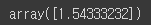
5 - 4. 조기종료
- 경사 하강법과 같은 반복적인 학습 알고리즘을 규제 방법
- 검증 에러가 최솟값에 도달하면 바로 훈련을 중지
np.random.seed(42)
m = 100
X = 6 * np.random.rand(m, 1) - 3
y = 2 + X + 0.5 * X**2 + np.random.randn(m, 1)

X_train, X_val, y_train, y_val = train_test_split(X[:50], y[:50].ravel(), test_size=0.5, random_state=10)


#조기 종료 구현 코드
from copy import deepcopy

poly_scaler = Pipeline([
        ("poly_features", PolynomialFeatures(degree=90, include_bias=False)),
        ("std_scaler", StandardScaler())
    ])

X_train_poly_scaled = poly_scaler.fit_transform(X_train)
X_val_poly_scaled = poly_scaler.transform(X_val)

sgd_reg = SGDRegressor(max_iter=1, tol=-np.infty, warm_start=True,
                       penalty=None, learning_rate="constant", eta0=0.0005, random_state=42)

minimum_val_error = float("inf")
best_epoch = None
best_model = None
for epoch in range(1000):
    sgd_reg.fit(X_train_poly_scaled, y_train)  # 중지된 곳에서 다시 시작합니다
    y_val_predict = sgd_reg.predict(X_val_poly_scaled)
    val_error = mean_squared_error(y_val, y_val_predict)
    if val_error < minimum_val_error:
        minimum_val_error = val_error
        best_epoch = epoch
        best_model = deepcopy(sgd_reg)
sgd_reg = SGDRegressor(max_iter=1, tol=-np.infty, warm_start=True,
penalty=None, learning_rate="constant", eta0=0.0005, random_state=42)
n_epochs = 500
train_errors, val_errors = [], []
for epoch in range(n_epochs):
sgd_reg.fit(X_train_poly_scaled, y_train)
y_train_predict = sgd_reg.predict(X_train_poly_scaled)
y_val_predict = sgd_reg.predict(X_val_poly_scaled)
train_errors.append(mean_squared_error(y_train, y_train_predict))
val_errors.append(mean_squared_error(y_val, y_val_predict))
best_epoch = np.argmin(val_errors)
best_val_rmse = np.sqrt(val_errors[best_epoch])
plt.annotate('Best model',
xy=(best_epoch, best_val_rmse),
xytext=(best_epoch, best_val_rmse + 1),
ha="center",
arrowprops=dict(facecolor='black', shrink=0.05),
fontsize=16,
)
best_val_rmse -= 0.03 # just to make the graph look better
plt.plot([0, n_epochs], [best_val_rmse, best_val_rmse], "k:", linewidth=2)
plt.plot(np.sqrt(val_errors), "b-", linewidth=3, label="Validation set")
plt.plot(np.sqrt(train_errors), "r--", linewidth=2, label="Training set")
plt.legend(loc="upper right", fontsize=14)
plt.xlabel("Epoch", fontsize=14)
plt.ylabel("RMSE", fontsize=14)
plt.show()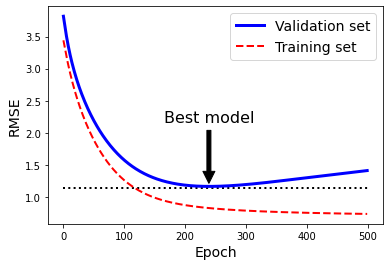
6. 로지스틱 회귀
- 샘플이 특정 클래스에 속할 확률을 추정
- 추정 확률이 50%을 넘으면 모델은 그 샘플이 해당 클래스에 속한다고 예측
6 - 1. 확률 추정
- 입력 특성의 가중치 합을 계산
- 선형 회귀처럼 바로 값을 출력하는 것이 아닌 결과값의 로지스틱 출력
- 로지스틱은 0과 1 사이의 값을 출력하는 시그모이드 함수
t = np.linspace(-10, 10, 100)
sig = 1 / (1 + np.exp(-t))
plt.figure(figsize=(9, 3))
plt.plot([-10, 10], [0, 0], "k-")
plt.plot([-10, 10], [0.5, 0.5], "k:")
plt.plot([-10, 10], [1, 1], "k:")
plt.plot([0, 0], [-1.1, 1.1], "k-")
plt.plot(t, sig, "b-", linewidth=2, label=r"$\sigma(t) = \frac{1}{1 + e^{-t}}$")
plt.xlabel("t")
plt.legend(loc="upper left", fontsize=20)
plt.axis([-10, 10, -0.1, 1.1])

plt.show()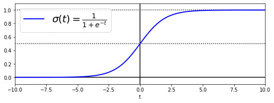
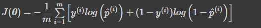
6 - 2. 훈련과 비용 함수
- 양성 샘플(y = 1)에 대해서는 높은 확률로 추정하는 모델의 파라미터 벡터를 찾음
- 음성 샘플(y = 0)에 대해서는 낮은 확률로 추정하는 모델의 파라미터 벡터를 찾음
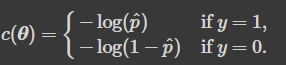
- 로지스틱 회귀의 비용 함수(로그 손실)
- 최솟값을 계산하는 해가 없음
- 볼록 함수이므로 경사 하강법 또는 최적화 알고리즘이 전역 최솟값을 찾음
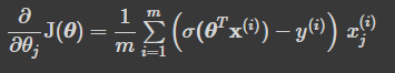
- 로지스틱 비용 함수의 편도 함수
- 각 샘플에 대한 예측 오차를 계산하고, j번째 특성값을 곱해서 모든 훈련 샘플에 대해 평균을 냄
- 모든 편도함수를 포함한 그에이디언트 벡터를 만들면 배치 경사 하강법 알고리즘 사용 가능
6 - 3. 결정 경계
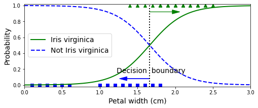
- iris data를 사용해 너비를 기반으로 iris-versicolor 종을 감지하는 분류기
from sklearn.datasets import iris_data
iris = iris_data()

list(iris.keys())

X = iris['data'][:, :3] # 꽃잎의 너비
y = (iris['target'] == 2).astype(int) #Iris-Virginica면 1, 그렇지 않으면 0
from sklearn.linear_model import LogisticRegression
model = LogisticRegression()
model.fit(X, y)
- 꽃잎의 너비가 0 ~ 3cm인 꽃에 대해 모델의 추정 확률을 계산
X_new = np.linspace(0, 3, 1000).reshape(-1, 1)
y_proba = log_reg.predict_proba(X_new)

plt.plot(X_new, y_proba[:, 1], "g-", linewidth=2, label="Iris virginica")
plt.plot(X_new, y_proba[:, 0], "b--", linewidth=2, label="Not Iris virginica")
X_new = np.linspace(0, 3, 1000).reshape(-1, 1)
y_proba = log_reg.predict_proba(X_new)
decision_boundary = X_new[y_proba[:, 1] >= 0.5][0]
plt.figure(figsize=(8, 3))
plt.plot(X[y==0], y[y==0], "bs")
plt.plot(X[y==1], y[y==1], "g^")
plt.plot([decision_boundary, decision_boundary], [-1, 2], "k:", linewidth=2)
plt.plot(X_new, y_proba[:, 1], "g-", linewidth=2, label="Iris virginica")
plt.plot(X_new, y_proba[:, 0], "b--", linewidth=2, label="Not Iris virginica")
plt.text(decision_boundary+0.02, 0.15, "Decision boundary", fontsize=14, color="k", ha="center")
plt.arrow(decision_boundary[0], 0.08, -0.3, 0, head_width=0.05, head_length=0.1, fc='b', ec='b')
plt.arrow(decision_boundary[0], 0.92, 0.3, 0, head_width=0.05, head_length=0.1, fc='g', ec='g')
plt.xlabel("Petal width (cm)", fontsize=14)
plt.ylabel("Probability", fontsize=14)
plt.legend(loc="center left", fontsize=14)
plt.axis([0, 3, -0.02, 1.02])
plt.show()- Iris-Verginia(삼각형)의 꽃잎 너비는 1.4 ~ 2.5cm에 분포
- 다른 붓꽃(사각형)은 너비가 더 작아 0.1 ~ 1.8cm에 분포
log_reg.predict([[1.7], [1.5]])
from sklearn.linear_model import LogisticRegression

X = iris["data"][:, (2, 3)]  # petal length, petal width
y = (iris["target"] == 2).astype(int)

log_reg = LogisticRegression(solver="lbfgs", C=10**10, random_state=42)
log_reg.fit(X, y)

x0, x1 = np.meshgrid(
        np.linspace(2.9, 7, 500).reshape(-1, 1),
        np.linspace(0.8, 2.7, 200).reshape(-1, 1),
    )
X_new = np.c_[x0.ravel(), x1.ravel()]

y_proba = log_reg.predict_proba(X_new)

plt.figure(figsize=(10, 4))
plt.plot(X[y==0, 0], X[y==0, 1], "bs")
plt.plot(X[y==1, 0], X[y==1, 1], "g^")

zz = y_proba[:, 1].reshape(x0.shape)
contour = plt.contour(x0, x1, zz, cmap=plt.cm.brg)


left_right = np.array([2.9, 7])
boundary = -(log_reg.coef_[0][0] * left_right + log_reg.intercept_[0]) / log_reg.coef_[0][1]

plt.clabel(contour, inline=1, fontsize=12)
plt.plot(left_right, boundary, "k--", linewidth=3)
plt.text(3.5, 1.5, "Not Iris virginica", fontsize=14, color="b", ha="center")
plt.text(6.5, 2.3, "Iris virginica", fontsize=14, color="g", ha="center")
plt.xlabel("Petal length", fontsize=14)
plt.ylabel("Petal width", fontsize=14)
plt.axis([2.9, 7, 0.8, 2.7])

plt.show()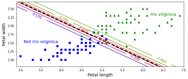
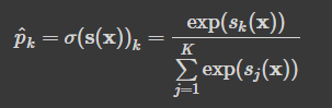
6 - 4. 소프트맥스 회귀
- 여러개의 이진 분류기를 훈련시켜 연결하지 않고 직접 다중 클래스를 지원하도록 일반화
- K: 클래스 수 / s(x): 샘플 x에 대한 각 클래스의 점수를 담은 벡터
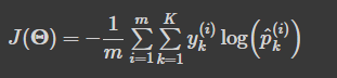
- 크로스 엔트로피 비용 함수
- 추정된 클래스의 확률이 타깃 클래스에 얼마나 잘 맞는지 측정하는 용도
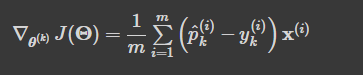
- 클래스 k에 대한 크로스 엔트로피의 그레이디언트 벡터
- Logistic Regression은 클래스가 둘 이상일 때 기본적으로 일대다 전략
- multi_class 매개변수를 multinomial로 바꾸면 소프트맥스 회귀 가능
- 추가적으로 solver 매개변수에 'lbfgs' 지정, 하이퍼파라미터 C 사용
X = iris["data"][:, (2, 3)]  # 꽃잎 길이, 꽃잎 너비
y = iris["target"]

softmax_reg = LogisticRegression(multi_class="multinomial",solver="lbfgs", C=10, random_state=42)
softmax_reg.fit(X, y)
softmax_reg.predict([[5, 2]])
softmax_reg.predict_proba([[5, 2]])
x0, x1 = np.meshgrid(
        np.linspace(0, 8, 500).reshape(-1, 1),
        np.linspace(0, 3.5, 200).reshape(-1, 1),
    )
X_new = np.c_[x0.ravel(), x1.ravel()]


y_proba = softmax_reg.predict_proba(X_new)
y_predict = softmax_reg.predict(X_new)

zz1 = y_proba[:, 1].reshape(x0.shape)
zz = y_predict.reshape(x0.shape)

plt.figure(figsize=(10, 4))
plt.plot(X[y==2, 0], X[y==2, 1], "g^", label="Iris virginica")
plt.plot(X[y==1, 0], X[y==1, 1], "bs", label="Iris versicolor")
plt.plot(X[y==0, 0], X[y==0, 1], "yo", label="Iris setosa")

from matplotlib.colors import ListedColormap
custom_cmap = ListedColormap(['#fafab0','#9898ff','#a0faa0'])

plt.contourf(x0, x1, zz, cmap=custom_cmap)
contour = plt.contour(x0, x1, zz1, cmap=plt.cm.brg)
plt.clabel(contour, inline=1, fontsize=12)
plt.xlabel("Petal length", fontsize=14)
plt.ylabel("Petal width", fontsize=14)
plt.legend(loc="center left", fontsize=14)
plt.axis([0, 7, 0, 3.5])

plt.show()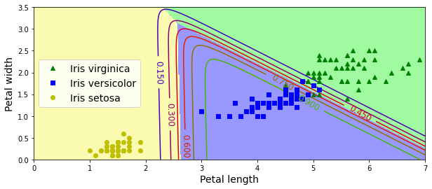
[머신러닝] 과대적합(overfitting)과 과소적합(underfitting)에 대해 알아보자!(+Early Stopping)
📚 목차 1. 과대적합 및 과소적합의 기본 개념 1.1. 과대적합(Overfitting)이란? 1.2. 과소적합(Underfitting)이란? 2. 과대적합 및 과소적합의 탐지 2.1. 분산과 편향 기반 탐지 2.2. 산점도 그래프 기반 탐지
heytech.tistory.com
핸즈온 머신러닝
머신러닝 전문가로 이끄는 최고의 실전 지침서 텐서플로 2.0을 반영한 풀컬러 개정판 『핸즈온 머신러닝』은 지능형 시스템을 구축하려면 반드시 알아야 할 머신러닝, 딥러닝 분야 핵심 개념과
book.naver.com
728x90
반응형
LIST
'Machine Learning의 민족 > 핸즈온 머신러닝' 카테고리의 다른 글
| < 핸즈온 머신러닝 - 차원 축소 > (0) | 2022.06.09 |
|---|---|
| < 핸즈온 머신러닝 - 앙상블 학습과 랜덤포레스트 > (0) | 2022.06.07 |
| < 핸즈온 머신러닝 - 결정 트리 > (0) | 2022.06.03 |
| < 핸즈온 머신러닝 - SVM > (0) | 2022.06.02 |
| < 핸즈온 머신러닝 - 분류 > (0) | 2022.05.10 |
'Machine Learning의 민족/핸즈온 머신러닝' Related Articles
more


Comments