
반응형
Notice
Recent Posts
Recent Comments
Link
| 일 | 월 | 화 | 수 | 목 | 금 | 토 |
|---|---|---|---|---|---|---|
| 1 | 2 | 3 | 4 | 5 | 6 | |
| 7 | 8 | 9 | 10 | 11 | 12 | 13 |
| 14 | 15 | 16 | 17 | 18 | 19 | 20 |
| 21 | 22 | 23 | 24 | 25 | 26 | 27 |
| 28 | 29 | 30 | 31 |
Tags
- 셸 소개
- DDL
- GPT4
- 생성다항식
- perfcc
- 셸 작업
- 머신러닝
- Tableau
- MYSQL
- 스크립트
- AWS
- centos7
- python
- 하둡
- .mongorc.js
- Retention
- 스머프 공격
- Power BI
- 비선형변환
- .perfcc
- PCA
- MNIST
- 도큐먼트
- 프롬프트 커스터마이징
- hadoop
- ubuntu
- AutoGPT
- 차원의 저주
- SQL
- 특징 교차
Archives
- Today
- Total
데이터의 민족
< 핸즈온 머신러닝 - 앙상블 학습과 랜덤포레스트 > 본문
728x90
반응형
SMALL
Chapter_7 앙상블 학습과 랜덤 포레스트.ipynb
Colaboratory notebook
colab.research.google.com
- 앙상블: 훈련 세트로부터 무작위로 각기 다른 서브셋을 만들어 일련의 결정 트리 분류기를 훈련
- 랜덤포레스트: 결정 트리의 앙상
1. 투표 기반 분류기
- 각 분류기의 예측을 모아서 가장 많이 선택된 클래스를 예측
- 다수결 투표로 정해지는 분류기를 직접 투표 분류기

1 - 1 예시
- 균형이 틀어진 동전을 10번 실험
- 던진 횟수가 증가할수록 51%에 수렴
import numpy as np

heads_proba = 0.51
coin_tosses = (np.random.rand(10000, 10) < heads_proba).astype(np.int32)
cumulative_heads_ratio = np.cumsum(coin_tosses, axis=0) / np.arange(1, 10001).reshape(-1, 1)
import matplotlib.pyplot as plt
plt.figure(figsize=(8,3.5))
plt.plot(cumulative_heads_ratio)
plt.plot([0, 10000], [0.51, 0.51], "k--", linewidth=2, label="51%")
plt.plot([0, 10000], [0.5, 0.5], "k-", label="50%")
plt.xlabel("Number of coin tosses")
plt.ylabel("Heads ratio")
plt.legend(loc="lower right")
plt.axis([0, 10000, 0.42, 0.58])
plt.show()
- 51% 정확도를 가진 1,000개의 분류기를 앙상블 모델을 구축할 경우, 75%의 정확도를 예측
- But) 모든 분류기가 완벽하게 독립적이고, 오차에 상관관계가 없어야 가능
1 - 2. make_moons 데이터 적용
from sklearn.datasets import make_moons
from sklearn.model_selection import train_test_split

X, y = make_moons(n_samples= 500, shuffle = True, noise=0.3, random_state = 42)
X_train, X_val, y_train, y_val = train_test_split(X, y, random_state = 42)
from sklearn.ensemble import RandomForestClassifier
from sklearn.ensemble import VotingClassifier
from sklearn.linear_model import LogisticRegression
from sklearn.svm import SVC
log_clf = LogisticRegression()
md_clf = RandomForestClassifier()
svm_clf = SVC(probability= True)
voting_clf = VotingClassifier(
estimators=[('lr', log_clf), ('rf', log_clf), ('svc', svm_clf)], voting="hard")
voting_clf.fit(X_train, y_train)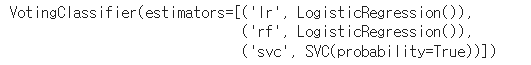
from sklearn.metrics import accuracy_score
for clf in (log_clf, md_clf, svm_clf, voting_clf):
  clf.fit(X_train, y_train)
  y_pred = clf.predict(X_val)
  print(clf.__class__.__name__, accuracy_score(y_val, y_pred))
1 - 3. 간접 투표(Soft Voting)
- 모든 분류기가 클래스의 확률을 예측할 수 있으면[predict_proba() 메서드를 보유], 개뱔 분류기의 예측을 평균 내어 확률이 가장 높은 클래스를 예측
- 확률이 높은 투표에 비중을 두기 때문에 hard보다 성능이 좋음
from sklearn.datasets import make_moons
from sklearn.model_selection import train_test_split

X, y = make_moons(n_samples= 500, shuffle = True, noise=0.3, random_state = 42)
X_train, X_val, y_train, y_val = train_test_split(X, y, random_state = 42)
from sklearn.ensemble import RandomForestClassifier
from sklearn.ensemble import VotingClassifier
from sklearn.linear_model import LogisticRegression
from sklearn.svm import SVC
log_clf = LogisticRegression()
md_clf = RandomForestClassifier()
svm_clf = SVC(probability= True)
voting_clf = VotingClassifier(
estimators=[('lr', log_clf), ('rf', log_clf), ('svc', svm_clf)], voting="soft")
voting_clf.fit(X_train, y_train)from sklearn.metrics import accuracy_score
for clf in (log_clf, md_clf, svm_clf, voting_clf):
clf.fit(X_train, y_train)
y_pred = clf.predict(X_val)
print(clf.__class__.__name__, accuracy_score(y_val, y_pred))
2. 배깅과 페이스팅
- 배깅: 훈련 세트에서 중복을 허용하여 샘플링하는 방식
- 페이스팅: 중복을 허용하지 않고 샘플링하는 방식
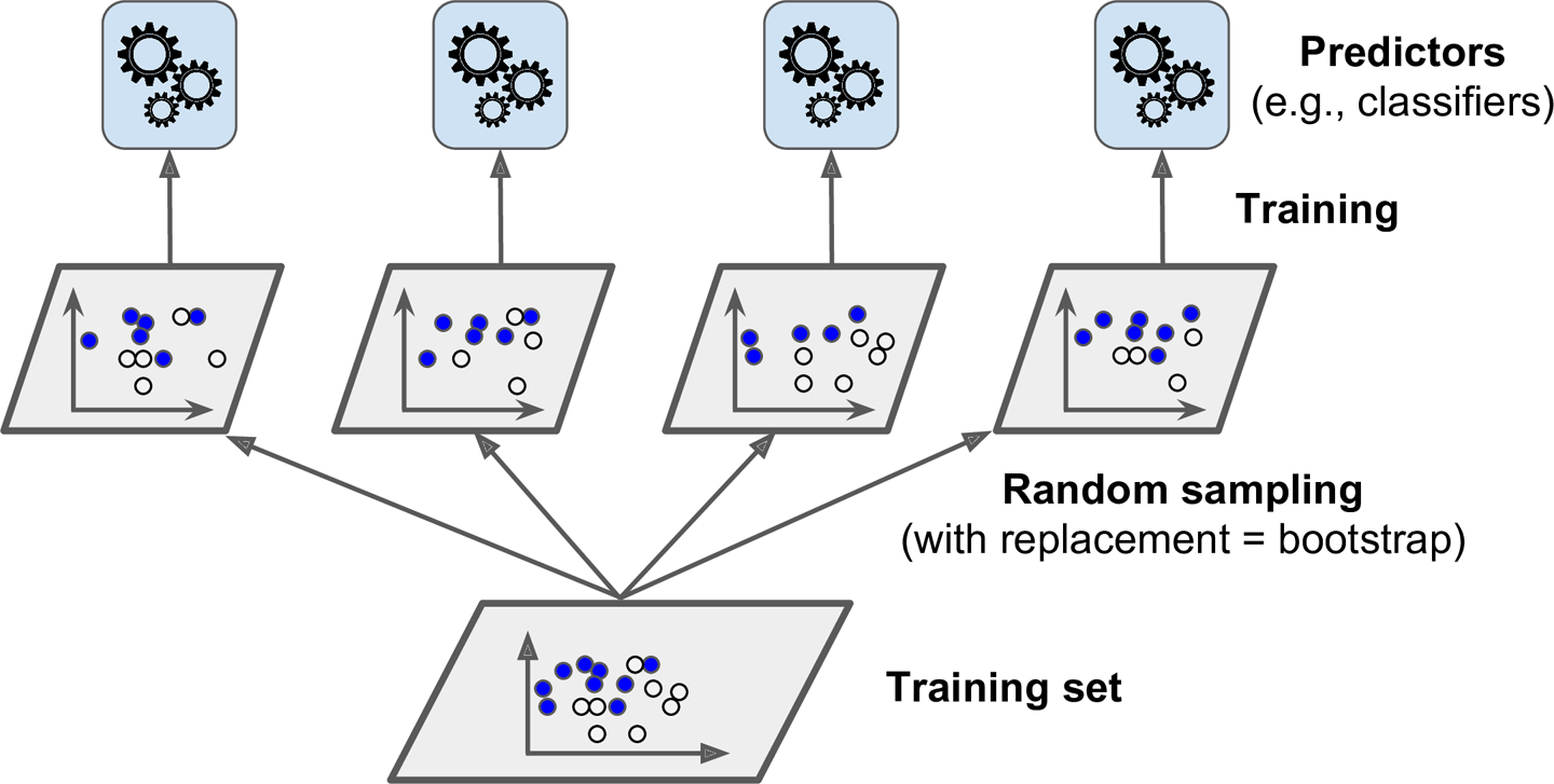
- 수집함수가 분류일 경우 통계적 최빈값
- 수집함수가 회귀일 경우 평균
2 - 1. 사이킷런의 배깅과 페이스팅
from sklearn.ensemble import BaggingClassifier
from sklearn.tree import DecisionTreeClassifier

bag_clf = BaggingClassifier(
  DecisionTreeClassifier(), n_estimators=500,
max_samples=100, bootstrap=True, n_jobs=-1)

bag_clf.fit(X_train, y_train)
y_pred = bag_clf.predict(X_val)

from sklearn.metrics import accuracy_score
print(accuracy_score(y_val, y_pred))
tree_clf = DecisionTreeClassifier(random_state=42)
tree_clf.fit(X_train, y_train)
y_pred_tree = tree_clf.predict(X_val)
print(accuracy_score(y_val, y_pred_tree))
from matplotlib.colors import ListedColormap

def plot_decision_boundary(clf, X, y, axes=[-1.5, 2.45, -1, 1.5], alpha=0.5, contour=True):
    x1s = np.linspace(axes[0], axes[1], 100)
    x2s = np.linspace(axes[2], axes[3], 100)
    x1, x2 = np.meshgrid(x1s, x2s)
    X_new = np.c_[x1.ravel(), x2.ravel()]
    y_pred = clf.predict(X_new).reshape(x1.shape)
    custom_cmap = ListedColormap(['#fafab0','#9898ff','#a0faa0'])
    plt.contourf(x1, x2, y_pred, alpha=0.3, cmap=custom_cmap)
    if contour:
        custom_cmap2 = ListedColormap(['#7d7d58','#4c4c7f','#507d50'])
        plt.contour(x1, x2, y_pred, cmap=custom_cmap2, alpha=0.8)
    plt.plot(X[:, 0][y==0], X[:, 1][y==0], "yo", alpha=alpha)
    plt.plot(X[:, 0][y==1], X[:, 1][y==1], "bs", alpha=alpha)
    plt.axis(axes)
    plt.xlabel(r"$x_1$", fontsize=18)
    plt.ylabel(r"$x_2$", fontsize=18, rotation=0)
fig, axes = plt.subplots(ncols=2, figsize=(10,4), sharey=True)
plt.sca(axes[0])
plot_decision_boundary(tree_clf, X, y)
plt.title("Decision Tree", fontsize=14)
plt.sca(axes[1])
plot_decision_boundary(bag_clf, X, y)
plt.title("Decision Trees with Bagging", fontsize=14)
plt.ylabel("")
plt.show()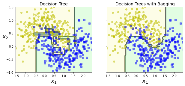
- 부트스트래핑은 각 예측기가 학습하는 서브셋에 다양성을 증가시키므로 배깅이 페이스팅보다 편향이 조금 더 높음
- But) 다양성을 추가한다는 것은 예측기들의 상관관계를 줄이므로 앙상블의 분산을 감소
- 평균적으로 배깅의 성능이 더 좋지만 시간의 여유가 있다면 둘 다 진행한 뒤에 비교하는 방향 추천
2 - 2. oob(out - of -bag) 평가
- BaggingClassifier는 기본값으로 중복을 허용하여(bootstrap = True) 훈련 세트의 크기만큼인 m개의 샘플을 선택
- 이는 평균적으로 각 예측기에 훈련 샘플의 63% 정도만 샘플링되는 것을 의미
- 선택되지 않은 훈련 샘플의 나머지 37%를 oob샘플이라고 지칭
- BaggingClassifier를 만들때 oob_score = True로 지정하면 자동으로 oob 평가를 평균화
bag_clf = BaggingClassifier(
    DecisionTreeClassifier(), n_estimators = 500,
    bootstrap = True, n_jobs = -1, oob_score = True)

bag_clf.fit(X_train, y_train)
print('BaggingClassifier는 테스트 세트에서 약',round(bag_clf.oob_score_, 4) , '정확도를 얻음')
from sklearn.metrics import accuracy_score
y_pred = bag_clf.predict(X_val)
accuracy_score(y_val, y_pred)
3. 랜덤 패치와 랜덤 서브스페이스
- BaggingClassifier에는 특성을 샘플링하는 max_features, bootstrap_features 매개변수 존재
- 랜덤 패치 방식: 훈련 특성과 샘플을 모두 샘플링하는 것
- 램덤 서브스페이스 방식: 훈련 샘플을 모두 사용하고, 특성은 샘플링하는 것
- 훈련 샘플: bootstrap = False, max_smaples = 1.0
- 특성 샘플링: bootstrap_features = True 그리고 /또는 max_features = 1.0으로 설정
4. 랜덤포레스트
- 배깅 방법을 적용한 결정 트리 앙상블
- max_smaples를 훈련 세트의 크기 결정
from sklearn.ensemble import RandomForestClassifier

rnd_clf = RandomForestClassifier(n_estimators = 500, max_leaf_nodes = 16, n_jobs = -1)
rnd_clf.fit(X_train, y_train)

y_pred = rnd_clf.predict(X_val)

bag_clf = BaggingClassifier(DecisionTreeClassifier(max_features = 'sqrt', max_leaf_nodes= 16), \
n_estimators = 500)
4 - 1. 엑스트라 트리
- 극단적으로 무작위한 트리의 랜덤 포레스트
- 편향이 늘어나지만 대신 분산을 낮춤
- 모든 노드에서 특성마다 가장 최적의 임곗값을 찾는 것이 트리 알고리즘에서 가장 시간이 많이 소요되는 작업 중 하나이므로 일반적인 랜덤 포레스트보다 빠름
- ExtraTreesClassifier를 사용
4 - 2. 특성 중요도
- 랜덤 포레스트의 장점: 상대적 중요도를 측정하기 쉬움
# iris_data 적용

from sklearn.datasets import load_iris
iris = load_iris()
rnd_clf = RandomForestClassifier(n_estimators= 500, n_jobs = -1)
rnd_clf.fit(iris['data'], iris['target'])

for name, score in zip(iris['feature_names'], rnd_clf.feature_importances_):
  print(name, score)
from sklearn.datasets import fetch_openml

mnist = fetch_openml('mnist_784', version=1)
mnist.target = mnist.target.astype(np.uint8)

rnd_clf = RandomForestClassifier(n_estimators=100, random_state=42)
rnd_clf.fit(mnist["data"], mnist["target"])
def plot_digit(data):
image = data.reshape(28, 28)
plt.imshow(image, cmap = mpl.cm.hot,
interpolation="nearest")
plt.axis("off")
plot_digit(rnd_clf.feature_importances_)
cbar = plt.colorbar(ticks=[rnd_clf.feature_importances_.min(), rnd_clf.feature_importances_.max()])
cbar.ax.set_yticklabels(['Not important', 'Very important'])
plt.show()
5. 부스팅
- 약한 학습기를 여러 개 연결하여 강한 학습기를 만드는 앙상블 방법
- 앞의 모델을 보완해나가면서 일련의 예측기를 학습
- 에이다부스트, 그레이디언트 부스트
5 - 1. AdaBoost
- 이전 예측기를 보완하는 새로운 예측기를 만드는 방법은 이전 모델이 과소적합한 훈련 샘플의 가중치를 더 높이는 것
- 새로운 예측기는 학습하기 어려운 샘플에 점점 더 맞춰지게 됨
-
- 에이다부스트의 기반이 되는 첫 번째 분류기를 훈련 세트에서 훈련시키고 예측을 생성
- 알고리즘이 잘못 분류된 샘플의 가중치를 상대적으로 높임
- 두 번째 분류기는 업데이트된 가중치를 사용해 훈련 세트에서 훈련하고 다시 예측을 생성
- 다시 가중치를 업데이트
-
from sklearn.ensemble import AdaBoostClassifier

ada_clf = AdaBoostClassifier(
    DecisionTreeClassifier(max_depth=1), n_estimators=200,
    algorithm="SAMME.R", learning_rate=0.5, random_state=42)
ada_clf.fit(X_train, y_train)

plot_decision_boundary(ada_clf, X, y)
m = len(X_train)

fig, axes = plt.subplots(ncols=2, figsize=(10,4), sharey=True)
for subplot, learning_rate in ((0, 1), (1, 0.5)):
    sample_weights = np.ones(m) / m
    plt.sca(axes[subplot])
    for i in range(5):
        svm_clf = SVC(kernel="rbf", C=0.2, gamma=0.6, random_state=42)
        svm_clf.fit(X_train, y_train, sample_weight=sample_weights * m)
        y_pred = svm_clf.predict(X_train)
        r = sample_weights[y_pred != y_train].sum() / sample_weights.sum() # equation 7-1
        alpha = learning_rate * np.log((1 - r) / r) # equation 7-2
        sample_weights[y_pred != y_train] *= np.exp(alpha) # equation 7-3
        sample_weights /= sample_weights.sum() # normalization step
        plot_decision_boundary(svm_clf, X, y, alpha=0.2)
        plt.title("learning_rate = {}".format(learning_rate), fontsize=16)
    if subplot == 0:
        plt.text(-0.7, -0.65, "1", fontsize=14)
        plt.text(-0.6, -0.10, "2", fontsize=14)
        plt.text(-0.5,  0.10, "3", fontsize=14)
        plt.text(-0.4,  0.55, "4", fontsize=14)
        plt.text(-0.3,  0.90, "5", fontsize=14)
    else:
        plt.ylabel("")


plt.show()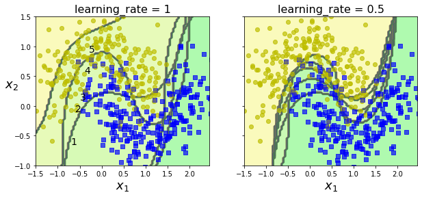
- AdaBoostClassifier의 기본 추정기
from sklearn.ensemble import AdaBoostClassifier

ada_clf = AdaBoostClassifier(
    DecisionTreeClassifier(max_depth = 1), n_estimators = 200,
    algorithm= 'SAMME.R', learning_rate = 0.5)

ada_clf.fit(X_train, y_train)
y_pred = ada_clf.predict(X_val)
accuracy_score(y_val, y_pred)
5 - 2. 그레이디언트 부스팅
- 앙상블 이전까지의 오차를 보정하도록 예측기를 순차적으로 추가
- 샘플의 가중치를 수정하는 AdaBoost와는 달리 이전 예측기가 만든 잔여 오차에 새로운 예측기를 학습
np.random.seed(42)
X = np.random.rand(100, 1) - 0.5
y = 3*X[:, 0]**2 + 0.05 * np.random.randn(100)

from sklearn.tree import DecisionTreeRegressor

tree_reg1 = DecisionTreeRegressor(max_depth=2, random_state=42)
tree_reg1.fit(X, y)

y2 = y - tree_reg1.predict(X)
tree_reg2 = DecisionTreeRegressor(max_depth=2, random_state=42)
tree_reg2.fit(X, y2)

y3 = y2 - tree_reg2.predict(X)
tree_reg3 = DecisionTreeRegressor(max_depth=2, random_state=42)
tree_reg3.fit(X, y3)
X_new = np.array([[0.8]])
y_pred = sum(tree.predict(X_new) for tree in (tree_reg1, tree_reg2, tree_reg3))
y_pred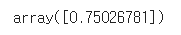
- 왼쪽: 학습한 모델들의 예측 / 오른쪽: 앙상블 모델 예측
def plot_predictions(regressors, X, y, axes, label=None, style="r-", data_style="b.", data_label=None):
    x1 = np.linspace(axes[0], axes[1], 500)
    y_pred = sum(regressor.predict(x1.reshape(-1, 1)) for regressor in regressors)
    plt.plot(X[:, 0], y, data_style, label=data_label)
    plt.plot(x1, y_pred, style, linewidth=2, label=label)
    if label or data_label:
        plt.legend(loc="upper center", fontsize=16)
    plt.axis(axes)
plt.figure(figsize=(11,11))
plt.subplot(321)
plot_predictions([tree_reg1], X, y, axes=[-0.5, 0.5, -0.1, 0.8], label="$h_1(x_1)$", style="g-", data_label="Training set")
plt.ylabel("$y$", fontsize=16, rotation=0)
plt.title("Residuals and tree predictions", fontsize=16)
plt.subplot(322)
plot_predictions([tree_reg1], X, y, axes=[-0.5, 0.5, -0.1, 0.8], label="$h(x_1) = h_1(x_1)$", data_label="Training set")
plt.ylabel("$y$", fontsize=16, rotation=0)
plt.title("Ensemble predictions", fontsize=16)
plt.subplot(323)
plot_predictions([tree_reg2], X, y2, axes=[-0.5, 0.5, -0.5, 0.5], label="$h_2(x_1)$", style="g-", data_style="k+", data_label="Residuals")
plt.ylabel("$y - h_1(x_1)$", fontsize=16)
plt.subplot(324)
plot_predictions([tree_reg1, tree_reg2], X, y, axes=[-0.5, 0.5, -0.1, 0.8], label="$h(x_1) = h_1(x_1) + h_2(x_1)$")
plt.ylabel("$y$", fontsize=16, rotation=0)
plt.subplot(325)
plot_predictions([tree_reg3], X, y3, axes=[-0.5, 0.5, -0.5, 0.5], label="$h_3(x_1)$", style="g-", data_style="k+")
plt.ylabel("$y - h_1(x_1) - h_2(x_1)$", fontsize=16)
plt.xlabel("$x_1$", fontsize=16)
plt.subplot(326)
plot_predictions([tree_reg1, tree_reg2, tree_reg3], X, y, axes=[-0.5, 0.5, -0.1, 0.8], label="$h(x_1) = h_1(x_1) + h_2(x_1) + h_3(x_1)$")
plt.xlabel("$x_1$", fontsize=16)
plt.ylabel("$y$", fontsize=16, rotation=0)
plt.show()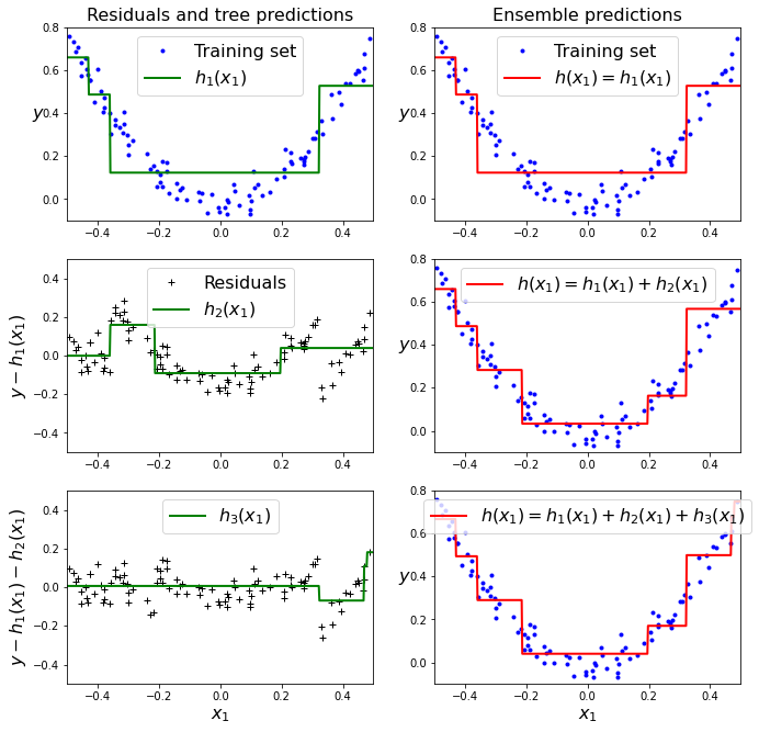
5 - 3. GBRT 앙상블
from sklearn.ensemble import GradientBoostingRegressor

gbrt = GradientBoostingRegressor(max_depth =2, n_estimators = 3, learning_rate = 1.0)
gbrt.fit(X, y)


gbrt_slow = GradientBoostingRegressor(max_depth=2, n_estimators=200, learning_rate=0.1, random_state=42)
gbrt_slow.fit(X, y)

fig, axes = plt.subplots(ncols=2, figsize=(10,4), sharey=True)

plt.sca(axes[0])
plot_predictions([gbrt], X, y, axes=[-0.5, 0.5, -0.1, 0.8], label="Ensemble predictions")
plt.title("learning_rate={}, n_estimators={}".format(gbrt.learning_rate, gbrt.n_estimators), fontsize=14)
plt.xlabel("$x_1$", fontsize=16)
plt.ylabel("$y$", fontsize=16, rotation=0)

plt.sca(axes[1])
plot_predictions([gbrt_slow], X, y, axes=[-0.5, 0.5, -0.1, 0.8])
plt.title("learning_rate={}, n_estimators={}".format(gbrt_slow.learning_rate, gbrt_slow.n_estimators), fontsize=14)
plt.xlabel("$x_1$", fontsize=16)


plt.show()
- learning_rate 매개변수가 각 트리의 기여 정도를 조절
- 0.1처럼 낮게 설정하면 앙상블을 훈련 세트에 학습시키기 위해 많은 트리가 필요하지만 일반적으로 예측의 성능은 좋아짐 -> 축소 규제 방법
5 - 4. 최적의 트리 수를 찾는 조기 종료 방법
import numpy as np
from sklearn.model_selection import train_test_split
from sklearn.metrics import mean_squared_error

X_train, X_val, y_train, y_val = train_test_split(X, y)

gbrt = GradientBoostingRegressor(max_depth = 2, n_estimators= 120)
gbrt.fit(X_train, y_train)

errors = [mean_squared_error(y_val, y_pred)
for y_pred in gbrt.staged_predict(X_val)]

bst_n_estimators = np.argmin(errors) + 1
gbrt_best = GradientBoostingRegressor(max_depth = 2, n_estimators = bst_n_estimators)
gbrt_best.fit(X_train, y_train)
# 왼쪽: 검증 오차 / 오른쪽: 최적 모델의 예측
min_error = np.min(errors)
plt.figure(figsize=(10, 4))
plt.subplot(121)
plt.plot(np.arange(1, len(errors) + 1), errors, "b.-")
plt.plot([bst_n_estimators, bst_n_estimators], [0, min_error], "k--")
plt.plot([0, 120], [min_error, min_error], "k--")
plt.plot(bst_n_estimators, min_error, "ko")
plt.text(bst_n_estimators, min_error*1.2, "Minimum", ha="center", fontsize=14)
plt.axis([0, 120, 0, 0.01])
plt.xlabel("Number of trees")
plt.ylabel("Error", fontsize=16)
plt.title("Validation error", fontsize=14)
plt.subplot(122)
plot_predictions([gbrt_best], X, y, axes=[-0.5, 0.5, -0.1, 0.8])
plt.title("Best model (%d trees)" % bst_n_estimators, fontsize=14)
plt.ylabel("$y$", fontsize=16, rotation=0)
plt.xlabel("$x_1$", fontsize=16)
plt.show()
- warm_start = True를 통해 기존 트리의 훈련을 유지하고, 훈련을 추가 가능
gbrt = GradientBoostingRegressor(max_depth = 2, warm_start = True)

min_val_error = float('inf')
error_going_up = 0

for n_estimators in range(1, 120):
  gbrt.n_estimators = n_estimators
  gbrt.fit(X_train, y_train)
  y_pred = gbrt.predict(X_val)
  val_error = mean_squared_error(y_val, y_pred)
  if val_error < min_val_error:
    min_val_error = val_error
    error_going_up = 0
  else:
    error_going_up += 1
    if error_going_up == 5:
      break #조기종료

print(gbrt.n_estimators)
print(gbrt.n_estimators) ==> 68
5 - 5. 확률적 그레이디언트 부스팅
- 예로 subsample = 0.25일 경우, 각 트리는 무작위로 선택된 25%의 훈련 샘플로 학습
- 편향이 높아지는 대신 분산이 낮아짐 + 훈련 속도 향상
import xgboost

xgb_reg = xgboost.XGBRFRegressor()
xgb_reg.fit(X_train, y_train)
y_pred = xgb_reg.predict(X_val)

# 조기 종료 기능
xgb_reg. fit(X_train, y_train,eval_set=[(X_val, y_val)], early_stopping_rounds=2)
y_pred = xgb_reg.predict(X_val)
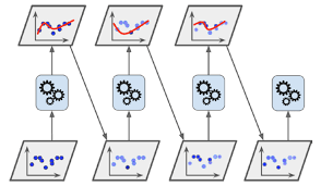
6. 스태킹(Stacked Generalization)
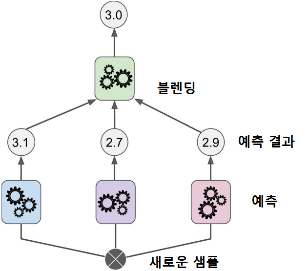

- 훈련 세트를 두 개의 서브셋으로 나눔
-
- 첫 번째 레이어의 예측을 훈련시키기 위해 사용
- 첫 번째 레이어의 예측기를 사용해 두 번째(홀드 아웃) 세트에 대한 예측을 생성
- 첫 번째 레이어의 예측기를 사용해 두 번째(홀드 아웃) 세트에 대한 예측을 생성
- 예측기들이 훈련하는 동안 보질 못했기에, 이때 생성된 예측은 완전히 새로운 것
- 홀드 아웃 세트의 각 샘플에 대해 3개의 예측값이 존재
- 타겟값은 그대로 쓰고 앞에서 예측한 값을 입력 특성으로 사용하는 새로운 훈련 세트를 만들 수 있음 --> 블랜더가 새 훈련 세트로 훈련
- 첫 번째 레이어의 예측을 가지고 타겟값을 예측

- 멀티 레이어 스태킹 앙상블 예측

핸즈온 머신러닝
머신러닝 전문가로 이끄는 최고의 실전 지침서 텐서플로 2.0을 반영한 풀컬러 개정판 『핸즈온 머신러닝』은 지능형 시스템을 구축하려면 반드시 알아야 할 머신러닝, 딥러닝 분야 핵심 개념과
book.naver.com
728x90
반응형
LIST
'Machine Learning의 민족 > 핸즈온 머신러닝' 카테고리의 다른 글
| < 핸즈온 머신러닝 - 비지도 학습1 - 군집 > (0) | 2022.06.14 |
|---|---|
| < 핸즈온 머신러닝 - 차원 축소 > (0) | 2022.06.09 |
| < 핸즈온 머신러닝 - 결정 트리 > (0) | 2022.06.03 |
| < 핸즈온 머신러닝 - SVM > (0) | 2022.06.02 |
| < 핸즈온 머신러닝 - 모델훈련 > (0) | 2022.05.17 |
'Machine Learning의 민족/핸즈온 머신러닝' Related Articles
more


Comments