
반응형
Notice
Recent Posts
Recent Comments
Link
| 일 | 월 | 화 | 수 | 목 | 금 | 토 |
|---|---|---|---|---|---|---|
| 1 | 2 | 3 | ||||
| 4 | 5 | 6 | 7 | 8 | 9 | 10 |
| 11 | 12 | 13 | 14 | 15 | 16 | 17 |
| 18 | 19 | 20 | 21 | 22 | 23 | 24 |
| 25 | 26 | 27 | 28 | 29 | 30 | 31 |
Tags
- Tableau
- DDL
- SQL
- PCA
- 스크립트
- 셸 소개
- GPT4
- 차원의 저주
- 도큐먼트
- 셸 작업
- MNIST
- 생성다항식
- .mongorc.js
- AutoGPT
- 프롬프트 커스터마이징
- AWS
- Retention
- python
- 하둡
- 특징 교차
- .perfcc
- MYSQL
- ubuntu
- perfcc
- 비선형변환
- Power BI
- centos7
- 머신러닝
- 스머프 공격
- hadoop
Archives
- Today
- Total
데이터의 민족
< 핸즈온 머신러닝 - 결정 트리 > 본문
728x90
반응형
SMALL
Chapter_6 결정 트리.ipynb
Colaboratory notebook
colab.research.google.com
- 분류, 회귀, 다중 출력 작업 가능
- 매우 복잡한 데이터셋 학습 가능
- 랜덤 포레스트의 기본 요소
1. 결정트리 학습과 시각화
from sklearn.datasets import load_iris
from sklearn.tree import DecisionTreeClassifier

iris = load_iris()

X = iris.data[:, 2:]
y = iris.target

tree_clf = DecisionTreeClassifier(max_depth = 2, random_state = 42)
tree_clf.fit(X, y)
from graphviz import Source
from sklearn.tree import export_graphviz
export_graphviz(
tree_clf,
out_file=os.path.join(IMAGES_PATH, "iris_tree.dot"),
feature_names=iris.feature_names[2:],
class_names=iris.target_names,
rounded=True,
filled=True
)
Source.from_file(os.path.join(IMAGES_PATH, "iris_tree.dot"))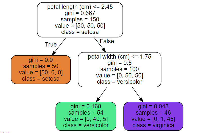
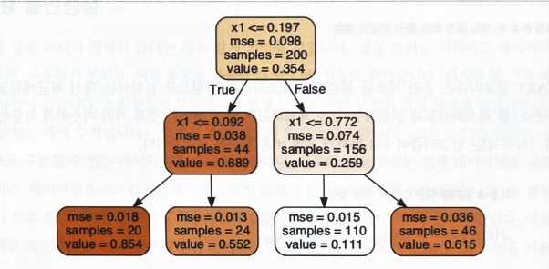
2. 예측하기
- 분류에서 루트 노드(깊이가 0인 맨 꼭대기의 노드)에서 시작
- 기준에 맞게 분류 진행
- 노드의 gini 속성은 불순도
- 한 노드의 샘플이 같은 클래스에 속해 있다면 순수 노드(gini = 0)
import matplotlib.pyplot as plt
import numpy as np
from matplotlib.colors import ListedColormap

def plot_decision_boundary(clf, X, y, axes=[0, 7.5, 0, 3], iris=True, legend=False, plot_training=True):
    x1s = np.linspace(axes[0], axes[1], 100)
    x2s = np.linspace(axes[2], axes[3], 100)
    x1, x2 = np.meshgrid(x1s, x2s)
    X_new = np.c_[x1.ravel(), x2.ravel()]
    y_pred = clf.predict(X_new).reshape(x1.shape)
    custom_cmap = ListedColormap(['#fafab0','#9898ff','#a0faa0'])
    plt.contourf(x1, x2, y_pred, alpha=0.3, cmap=custom_cmap)
    if not iris:
        custom_cmap2 = ListedColormap(['#7d7d58','#4c4c7f','#507d50'])
        plt.contour(x1, x2, y_pred, cmap=custom_cmap2, alpha=0.8)
    if plot_training:
        plt.plot(X[:, 0][y==0], X[:, 1][y==0], "yo", label="Iris setosa")
        plt.plot(X[:, 0][y==1], X[:, 1][y==1], "bs", label="Iris versicolor")
        plt.plot(X[:, 0][y==2], X[:, 1][y==2], "g^", label="Iris virginica")
        plt.axis(axes)
    if iris:
        plt.xlabel("Petal length", fontsize=14)
        plt.ylabel("Petal width", fontsize=14)
    else:
        plt.xlabel(r"$x_1$", fontsize=18)
        plt.ylabel(r"$x_2$", fontsize=18, rotation=0)
    if legend:
        plt.legend(loc="lower right", fontsize=14)

plt.figure(figsize=(8, 4))
plot_decision_boundary(tree_clf, X, y)
plt.plot([2.45, 2.45], [0, 3], "k-", linewidth=2)
plt.plot([2.45, 7.5], [1.75, 1.75], "k--", linewidth=2)
plt.plot([4.95, 4.95], [0, 1.75], "k:", linewidth=2)
plt.plot([4.85, 4.85], [1.75, 3], "k:", linewidth=2)
plt.text(1.40, 1.0, "Depth=0", fontsize=15)
plt.text(3.2, 1.80, "Depth=1", fontsize=13)
plt.text(4.05, 0.5, "(Depth=2)", fontsize=11)


plt.show()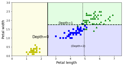
- 굵은 수직선이 루트 노즈(깊이 0)의 결정 경계(꽃잎 길이 = 2.45)를 나타냄
- 왼쪽: 순수 노드의 영역
- 오른쪽: 순수 노드의 영역이 아니기에 꽃잎 너비 1.75에서 나누어짐
- max_depth = 2이기에 추가 분할 없음
2 - 1. 블랙 박스와 화이트 박스
- 화이트 박스: 결정 트리와 같이 직곽적이고 결정 방식의 이해가 쉬운 모델
- 블랙박스: 랜덤 포레스트나 신경망 같이 알고리즘의 성능이 뛰어나고 예측을 만드는 연산 과정이 쉽게 확인 가능
- But) 설명이 어려움
3. 클래스 확률의 추정
- 예시) 깊이가 5, 너비가 1.5인 꽃잎
tree_clf.predict_proba([[5, 1.5]]), tree_clf.predict([[5, 1.5]])
4. CART 훈련 알고리즘
- Decision Tree 성장 위해 사용
- 탐욕적 알고리즘으로, 맨 위 루트 노드에서 최적의 분할을 찾으며 이어지는 각 단계에서 이 과정을 반복
- But) 현재 단계의 분할이 몇 단계를 거쳐 가장 낮은 불순도로 이어질 수 있는지에 대한 고려 없음 + 최적의 솔루션 보장 없음
- 탐욕적 알고리즘은 납득할 만한 좋은 솔루션 정도

5. 계산 복잡도
- 결정 트리를 탐색하기 위해서는 O(log2(m))개의 노드를 거쳐야함
- 하나의 특성값만 예측시 확인하기 때문에 특성 수와 무관하며, 큰 훈련 세트를 다룰 때도 예측 속도가 매우 빠름
- 훈련 세트가 수천 개 이하일 경우 사이킷런은 presort = True로 지정하면 훈련 속도를 높일 수 있음
6. 지니 불순도 또는 엔트로피?
- default는 지니 지수이지만, criterion 매개변수를 'entropy'로 지정하면 엔트로피 불순도를 사용
- 엔트로피는 분자의 무질서함을 측정하는 것으로 원래 열역학의 개념, 분자가 안정되고 질서 정연하면 엔트로피가 0에 가까움
- 지니와 엔트로피의 큰 차이는 없음, 지니 분순도가 좀 더 빠른정도
- 가장 빈도가 높은 클래스를 한쪽 가지로 고립시키는 경향이 있는 지니 불순도에 반해, 엔트로피는 좀 더 균형 잡힌 트리를 생성
7. 규제 매개변수
- 결정 트리는 훈련 데이터에 대한 제약 사항이 거의 없음
- 결정 트리는 파라미터가 보통 많지만, 수가 결정되지 않기 때문에 이런 모델을 비파라미터 모델이라고 지칭
- But) 결정 트리의 과적합을 막기 위해 자유도에 대한 제한 필요 있음
- 사이킷런에서 결정 트리에 대한 규제변수는 max_depth
- min_으로 시작하는 매개변수를 증가시키거나 max_로 시작하는 매개변수를 감소시키면 모델에 대한 규제가 커짐
- min_samples_split (분할되기 위해 노드가 가져야 하는 최소 샘플 수)
- min_samples_leaf (리프 노드가 가지고 있어야 할 최소 샘플 수)
- min_weight_fraction_leaf(min_samples_leaf와 같지만 가중치가 부여된 전체 샘플 수에서의 비율)
- max_leaf_nodes(리프 노드의 최대 수)
- max_features (각 노드에서 분할에 사용할 특성의 최대 수)
# 오른쪽 결정 트리는 min_samples_leaf = 4로 지정 훈련
from sklearn.datasets import make_moons
Xm, ym = make_moons(n_samples=100, noise=0.25, random_state=53)

deep_tree_clf1 = DecisionTreeClassifier(random_state=42)
deep_tree_clf2 = DecisionTreeClassifier(min_samples_leaf=4, random_state=42)
deep_tree_clf1.fit(Xm, ym)
deep_tree_clf2.fit(Xm, ym)

fig, axes = plt.subplots(ncols=2, figsize=(10, 4), sharey=True)
plt.sca(axes[0])
plot_decision_boundary(deep_tree_clf1, Xm, ym, axes=[-1.5, 2.4, -1, 1.5], iris=False)
plt.title("No restrictions", fontsize=16)
plt.sca(axes[1])
plot_decision_boundary(deep_tree_clf2, Xm, ym, axes=[-1.5, 2.4, -1, 1.5], iris=False)
plt.title("min_samples_leaf = {}".format(deep_tree_clf2.min_samples_leaf), fontsize=14)
plt.ylabel("")


plt.show()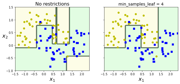
8. 회귀
# 2차식으로 만든 데이터셋 + 잡음
np.random.seed(42)
m = 200
X = np.random.rand(m, 1)
y = 4 * (X - 0.5) ** 2
y = y + np.random.randn(m, 1) / 10
from sklearn.tree import DecisionTreeRegressor
tree_reg = DecisionTreeRegressor(max_depth = 2)
tree_reg.fit(X, y)- 만약 x1 = 0.6인 타깃값을 예측한다고 가정
- 루트 노드부터 시작, 트리를 순회하면 value = 0.111인 리프 노드에 도달
- 이 리프 노드에 있는 110개 훈련 샘플의 평균 타깃값이 예측값
- 110개 샘플에 대한 MSE(평균제곱오차)를 계산하면 0.015
from sklearn.tree import DecisionTreeRegressor

tree_reg1 = DecisionTreeRegressor(random_state=42, max_depth=2)
tree_reg2 = DecisionTreeRegressor(random_state=42, max_depth=3)
tree_reg1.fit(X, y)
tree_reg2.fit(X, y)

def plot_regression_predictions(tree_reg, X, y, axes=[0, 1, -0.2, 1], ylabel="$y$"):
    x1 = np.linspace(axes[0], axes[1], 500).reshape(-1, 1)
    y_pred = tree_reg.predict(x1)
    plt.axis(axes)
    plt.xlabel("$x_1$", fontsize=18)
    if ylabel:
        plt.ylabel(ylabel, fontsize=18, rotation=0)
    plt.plot(X, y, "b.")
    plt.plot(x1, y_pred, "r.-", linewidth=2, label=r"$\hat{y}$")

fig, axes = plt.subplots(ncols=2, figsize=(10, 4), sharey=True)
plt.sca(axes[0])
plot_regression_predictions(tree_reg1, X, y)
for split, style in ((0.1973, "k-"), (0.0917, "k--"), (0.7718, "k--")):
    plt.plot([split, split], [-0.2, 1], style, linewidth=2)
plt.text(0.21, 0.65, "Depth=0", fontsize=15)
plt.text(0.01, 0.2, "Depth=1", fontsize=13)
plt.text(0.65, 0.8, "Depth=1", fontsize=13)
plt.legend(loc="upper center", fontsize=18)
plt.title("max_depth=2", fontsize=14)

plt.sca(axes[1])
plot_regression_predictions(tree_reg2, X, y, ylabel=None)
for split, style in ((0.1973, "k-"), (0.0917, "k--"), (0.7718, "k--")):
    plt.plot([split, split], [-0.2, 1], style, linewidth=2)
for split in (0.0458, 0.1298, 0.2873, 0.9040):
    plt.plot([split, split], [-0.2, 1], "k:", linewidth=1)
plt.text(0.3, 0.5, "Depth=2", fontsize=13)
plt.title("max_depth=3", fontsize=14)


plt.show()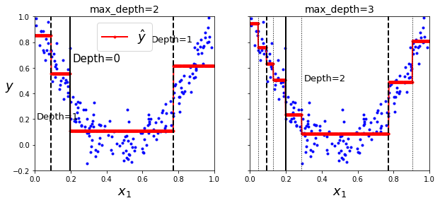
tree_reg1 = DecisionTreeRegressor(random_state=42)
tree_reg2 = DecisionTreeRegressor(random_state=42, min_samples_leaf=10)
tree_reg1.fit(X, y)
tree_reg2.fit(X, y)

x1 = np.linspace(0, 1, 500).reshape(-1, 1)
y_pred1 = tree_reg1.predict(x1)
y_pred2 = tree_reg2.predict(x1)

fig, axes = plt.subplots(ncols=2, figsize=(10, 4), sharey=True)

plt.sca(axes[0])
plt.plot(X, y, "b.")
plt.plot(x1, y_pred1, "r.-", linewidth=2, label=r"$\hat{y}$")
plt.axis([0, 1, -0.2, 1.1])
plt.xlabel("$x_1$", fontsize=18)
plt.ylabel("$y$", fontsize=18, rotation=0)
plt.legend(loc="upper center", fontsize=18)
plt.title("No restrictions", fontsize=14)

plt.sca(axes[1])
plt.plot(X, y, "b.")
plt.plot(x1, y_pred2, "r.-", linewidth=2, label=r"$\hat{y}$")
plt.axis([0, 1, -0.2, 1.1])
plt.xlabel("$x_1$", fontsize=18)
plt.title("min_samples_leaf={}".format(tree_reg2.min_samples_leaf), fontsize=14)

plt.show()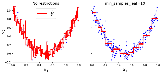
9. 불안정성
- 계단 모양의 결정 경계 생성(모든 분할은 축에 수직)
- So) 훈련 세트의 회전에 민감
np.random.seed(6)
Xs = np.random.rand(100, 2) - 0.5
ys = (Xs[:, 0] > 0).astype(np.float32) * 2

angle = np.pi / 4
rotation_matrix = np.array([[np.cos(angle), -np.sin(angle)], [np.sin(angle), np.cos(angle)]])
Xsr = Xs.dot(rotation_matrix)

tree_clf_s = DecisionTreeClassifier(random_state=42)
tree_clf_s.fit(Xs, ys)
tree_clf_sr = DecisionTreeClassifier(random_state=42)
tree_clf_sr.fit(Xsr, ys)

fig, axes = plt.subplots(ncols=2, figsize=(10, 4), sharey=True)
plt.sca(axes[0])
plot_decision_boundary(tree_clf_s, Xs, ys, axes=[-0.7, 0.7, -0.7, 0.7], iris=False)
plt.sca(axes[1])
plot_decision_boundary(tree_clf_sr, Xsr, ys, axes=[-0.7, 0.7, -0.7, 0.7], iris=False)
plt.ylabel("")

plt.show()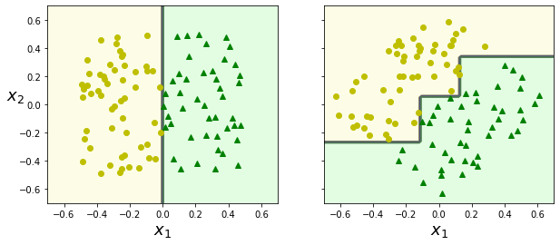
- 왼쪽 결정 트리는 간단한 선형 분류
- 오른쪽 결정 트리는 45도를 회전한 데이터셋을 사용
- 더 좋은 방향으로 회전 시키는 방법: PCA(주성분분석)
핸즈온 머신러닝
머신러닝 전문가로 이끄는 최고의 실전 지침서 텐서플로 2.0을 반영한 풀컬러 개정판 『핸즈온 머신러닝』은 지능형 시스템을 구축하려면 반드시 알아야 할 머신러닝, 딥러닝 분야 핵심 개념과
book.naver.com
728x90
반응형
LIST
'Machine Learning의 민족 > 핸즈온 머신러닝' 카테고리의 다른 글
| < 핸즈온 머신러닝 - 차원 축소 > (0) | 2022.06.09 |
|---|---|
| < 핸즈온 머신러닝 - 앙상블 학습과 랜덤포레스트 > (0) | 2022.06.07 |
| < 핸즈온 머신러닝 - SVM > (0) | 2022.06.02 |
| < 핸즈온 머신러닝 - 모델훈련 > (0) | 2022.05.17 |
| < 핸즈온 머신러닝 - 분류 > (0) | 2022.05.10 |
'Machine Learning의 민족/핸즈온 머신러닝' Related Articles
more


Comments