
반응형
Notice
Recent Posts
Recent Comments
Link
| 일 | 월 | 화 | 수 | 목 | 금 | 토 |
|---|---|---|---|---|---|---|
| 1 | 2 | 3 | ||||
| 4 | 5 | 6 | 7 | 8 | 9 | 10 |
| 11 | 12 | 13 | 14 | 15 | 16 | 17 |
| 18 | 19 | 20 | 21 | 22 | 23 | 24 |
| 25 | 26 | 27 | 28 | 29 | 30 | 31 |
Tags
- MYSQL
- Retention
- AWS
- ubuntu
- 프롬프트 커스터마이징
- SQL
- centos7
- 머신러닝
- 특징 교차
- .perfcc
- 하둡
- 도큐먼트
- 셸 소개
- Tableau
- 스머프 공격
- 비선형변환
- AutoGPT
- 스크립트
- 차원의 저주
- 생성다항식
- DDL
- hadoop
- 셸 작업
- Power BI
- .mongorc.js
- PCA
- MNIST
- perfcc
- GPT4
- python
Archives
- Today
- Total
데이터의 민족
< 핸즈온 머신러닝 - 분류 > 본문
728x90
반응형
SMALL
Chapter_3 분류.ipynb
Colaboratory notebook
colab.research.google.com
1. MNIST
1 - 1. 데이터 불러오기
from sklearn.datasets import fetch_openml
mnist = fetch_openml('mnist_784', version =1, as_frame = False)
mnist.keys()
1 - 2. 배열확인
- 이미지가 70,000개이며, 각 이미지에는 784개의 특성 존재(28 X 28 픽셀)
X, y = mnist['data'], mnist['target']
print(X.shape)
print(y.shape)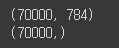
1 - 3. 이미지 예시 출력
import matplotlib as mpl
import matplotlib.pyplot as plt

some_digit = X[0]
some_digit_image = some_digit.reshape(28, 28)

plt.imshow(some_digit_image, cmap = 'binary')
plt.axis('off')
plt.show

# 실제 레이블 확인
print('실제 레이블 :', y[0])
1 - 4. y 정수로 변환(레이블이 문자열이기 때문)
import numpy as np
y = y.astype(np.int8)
y
1 - 5. train, test 셋 분류
X_train, X_val, y_train, y_val = X[:60000], X[60000:], y[:60000], y[60000:]
2. 이진 분류기 훈련
- '5'와 '5 아님' 두 개의 클래스를 구분
2 - 1. 타깃 벡터 생성
y_train_5 = (y_train == 5) # 5는 True고, 다른 숫자는 모두 False
y_test_5 = (y_val == 5)
2 - 2. Scikit-Learn의 SGDClassifier 클래스를 사용해 확률적 경사 하강법 적용
- 큰 데이터 셋을 효율적으로 처리
- 한 번에 하나씩 훈련 샘플을 독립적으로 처리
- SGDClassifier은 훈련하는 데 확룰적(무작위)이기에, 결과 재현을 위한 매개변수 지정
from sklearn.linear_model import SGDClassifier
model = SGDClassifier(random_state= 42)
model.fit(X_train, y_train)
model.predict([some_digit])
3. 성능 측정
- StratifiedKfolds는 클래스별 비율이 유지되도록 폴드를 만들기 위해 계층적 샘플링 수행
- 매 반복에서 분류기 객체를 복제하여 훈련 폴드로 훈련시키고 테스트 폴드로 예측
- 올바른 예측의 수를 세어 정확한 예측의 비율을 출력
from sklearn.model_selection import StratifiedKFold
from sklearn.base import clone

skfolds = StratifiedKFold(n_splits =3, random_state = 42, shuffle = True)

for train_index, val_index in skfolds.split(X_train, y_train_5):
  clone_model = clone(model)
  X_train_folds = X_train[train_index]
  y_train_folds = y_train_5[train_index]

  X_val_folds = X_train[val_index]
  y_val_folds = y_train_5[val_index]

  clone_model.fit(X_train_folds, y_train_folds)
  y_pred = clone_model.predict(X_val_folds)
  n_correct = sum(y_pred == y_val_folds)
  print(n_correct / len(y_pred))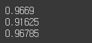
3 - 1. cross_val_score 함수 평가
from sklearn.model_selection import cross_val_score
cross_val_score(model, X_train, y_train_5, cv =3, scoring = 'accuracy')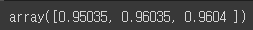
from sklearn.base import BaseEstimator

class Never5Classifier(BaseEstimator):
  def fit(self, X, y = None):
    return self
  def predict(self, X):
    return np.zeros((len(X), 1), dtype = bool)

# 정확도 예측
never_5_model = Never5Classifier()
cross_val_score(never_5_model, X_train, y_train_5, cv = 3, scoring = 'accuracy')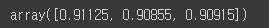
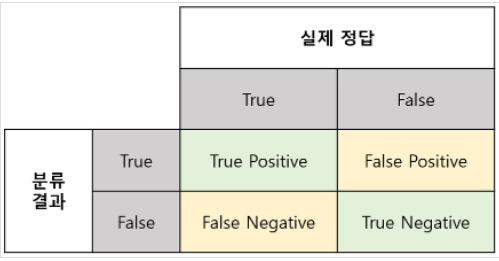
4. 오차 행렬
- 분류기의 성능 평가
- 먼저 실제 타겟과 비교할 수 있는 예측값을 생성
- 교차 검증을 수행하지만, 평가 점수를 반환하지 않고 각 테스트 폴드에서 얻은 예측 반환
from sklearn.model_selection import cross_val_predict
y_train_pred = cross_val_predict(clone_model, X_train, y_train_5, cv = 3)
- 완벽한 분류기라면 진짜 양성과 진짜 음성만 가지고 있을 것이므로 왼쪽 위에서 오른쪽 아래로 0이 아닌 값
from sklearn.metrics import confusion_matrix
confusion_matrix(y_train_5, y_train_pred)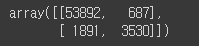
y_train_perfect_predictions = y_train_5
confusion_matrix(y_train_5, y_train_perfect_predictions)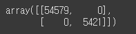
5. 정밀도 / 재현율
5 - 1. 정밀도
- 양성 예측의 정확도
- TP: 진짜 양성 예측의 정확도 / FP: 거짓 양수의 수
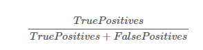
from sklearn.metrics import precision_score
precision_score(y_train_5, y_train_pred)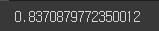
5 - 2. 재현율 == 민감도
- FN: 거짓 음성의 수
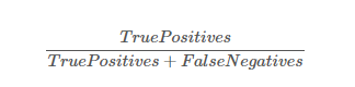
from sklearn.metrics import accuracy_score, recall_score
print(recall_score(y_train_5, y_train_pred))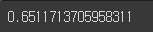
5 - 3. f1_score

from sklearn.metrics import f1_score
f1_score(y_train_5, y_train_pred)
6. 정밀도 / 재현율 트레이드오프
- decision_function: 각 샘플의 점수를 얻음
y_scores = clone_model.decision_function([some_digit])
y_scores

threshold = 0
y_some_digit_pred = (y_scores > threshold)
y_some_digit_pred
6 - 1. 임계값 상승
- 재현율 감소
threshold = 8000
y_some_digit_pred = (y_scores > threshold)
y_some_digit_pred
6 - 2. 적절한 임계값 탐색
y_scores = cross_val_predict(clone_model, X_train, y_train_5, cv =3, method = 'decision_function')


from sklearn.metrics import precision_recall_curve
precisions, recalls, thresholds = precision_recall_curve(y_train_5, y_scores)


# 정밀도 곡선이 울퉁불퉁한 이유는 임계값을 올리더라도 정밀도가 낮아지는 경우 발생
# 왜냐하면 임계값을 올릴수록 반비례 관계이기 때문

def plot_precision_recall_vs_threshold(precisions, recalls, thresholds):
  plt.plot(thresholds, precisions[:-1], 'b--',label = 'Precision')
  plt.plot(thresholds, recalls[:-1], 'g-',label = 'Recall')
  plt.grid(True, color = 'gray',linestyle = '--')
  plt.legend()

plot_precision_recall_vs_threshold(precisions, recalls, thresholds)
plt.show()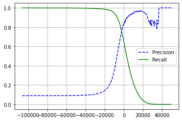
# np.argmax()는 최댓값의 첫 번째 인덱스 반환
threshold_90_precision = thresholds[np.argmax(precisions >= 0.90)]
y_train_pred_90 = (y_scores >= threshold_90_precision)


# 정밀도를 90% 달성: 임계값을 향상
# 그러나 재현율이 너무 낮다면 유용하지 않은 정밀도 분류기

print(precision_score(y_train_5, y_train_pred_90))
print(recall_score(y_train_5, y_train_pred_90))
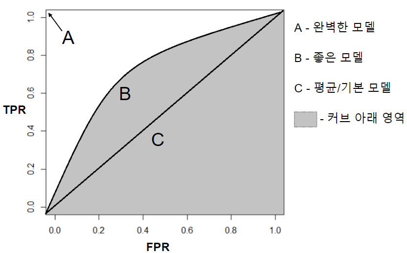
7. ROC(수신기 조작 특성) 곡선
- Receiver Operating Characteristic
- 거짓 양성 비율(FPR)에 대한 진짜 양성 비율(TPR)의 곡선
- 민감도(재현율)에 대한 1 - 특이도
from sklearn.metrics import roc_curve
fpr, tpr, threshold = roc_curve(y_train_5, y_scores)

def plot_roc_curve(fpr, tpr, label = None):
  plt.plot(fpr, tpr, linewidth = 2, label = label)
  plt.plot([0,1], [0,1], 'k--')

plot_roc_curve(fpr, tpr)
plt.show()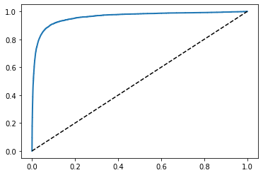
7 - 1. AUC(곡선 아래의 면적)
- 완벽한 분류기는 ROC의 AUC가 1
- 완전한 랜덤 분류기는 0.5
from sklearn.metrics import roc_auc_score
roc_auc_score(y_train_5, y_scores)
7 - 2. RandomForestClassifier을 사용한 ROC, AUC
- RandomForestClassifier에는 decision_function() 기능이 없어 predict_prob() 사용
- predict_proba(): 샘플이 행, 클래스가 열이고 샘플이 주어진 클래스에 속할 확률을 담은 배열
- 예를 들어 '어떤 이미지가 5일 확룰 70%'
from sklearn.ensemble import RandomForestClassifier

model = RandomForestClassifier(random_state = 42)
y_prebas_forest = cross_val_predict(model, X_train, y_train_5, cv = 3, method = 'predict_proba')
y_scores_forest = y_prebas_forest[:,1]
fpr_forest, tpr_forest, thresholds_forest = roc_curve(y_train_5, y_scores_forest)plt.plot(fpr, tpr, 'b:', label = 'SGD')
plot_roc_curve(fpr_forest, tpr_forest, 'RandomForest')
plt.legend(loc = 'lower right')
plt.show()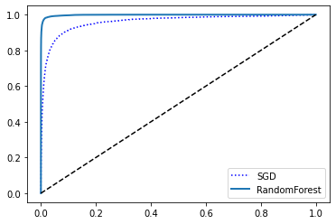
# RandomForest 점수
roc_auc_score(y_train_5, y_scores_forest)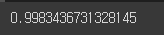
8. 다중 분류
- SGD, RandomForest, Naive Bayes 분류기는 여러 개의 클래스 직접 처리
- Logistic, SVM 분류기는 이진 분류만 가능
- OVR, OAR: 이미지를 분류할 때 각 분류기의 결정 점수 중에서 가장 높은 것을 클래스로 선택
- OVE: 0과 1 구별, 0과 2 구별, 1과 2 구별 등과 같이 각 숫자의 조합마다 이진 분류기를 훈련
- 클래스가 N개일 경우 분류기는 N*(N-1)/2개
from sklearn.svm import SVC

svm_clf = SVC()
svm_clf.fit(X_train, y_train) #5를 구분한 y_train_5가 아닌 0 - 9가 포함된 원래의 타깃 클래스 훈련
svm_clf.predict([some_digit])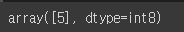
some_digit_scores = svm_clf.decision_function([some_digit])
some_digit_scores
np.argmax([some_digit_scores])
8 - 2. SVC기반 OVR 다중 분류기
from sklearn.multiclass import OneVsRestClassifier
ovr_clf = OneVsRestClassifier(SVC())
ovr_clf.fit(X_train, y_train)
ovr_clf.predict([some_digit])
len(ovr_clf.estimators_)
8 - 3. SGDC 훈련
- 직접 샘플을 다중 클래스로 분류 가능
from sklearn.linear_model import SGDClassifier
sgd_clf = SGDClassifier()
sgd_clf.fit(X_train, y_train)
sgd_clf.predict([some_digit])
len(sgd_clf.estimators_)

cross_val_score(sgd_clf, X_train, y_train, cv =3, scoring = 'accuracy')
8 - 4. 표준화
from sklearn.preprocessing import StandardScaler
from sklearn.model_selection import cross_val_score
from sklearn.linear_model import SGDClassifier
sgd_clf = SGDClassifier()

scaler = StandardScaler()
X_train_scaled = scaler.fit_transform(X_train.astype(np.float64))
cross_val_score(sgd_clf, X_train_scaled, y_train, cv = 3, scoring = 'accuracy')
9. 에러 분석
9 - 1. 오차 행렬 분석
y_train_pred = cross_val_predict(sgd_clf, X_train_scaled, y_train, cv =3)
conf_mx = confusion_matrix(y_train, y_train_pred)
conf_mx

plt.matshow(conf_mx, cmap = cm.gray)
plt.show()
# 그래프의 에러에 초점
# 오차 행렬의 각 값을 대응되는 클래스의 이미지 개수로 나누어 에러 비율 비교
# 개수로 비교하게 된다면 이미지가 많은 클래스가 상대적으로 나쁜 결과 출력
row_sums = conf_mx.sum(axis = 1, keepdims = True)
norm_conf_mx = conf_mx / row_sums
np.fill_diagonal(norm_conf_mx, 0)
plt.matshow(norm_conf_mx, cmap = plt.cm.gray)
plt.show()
10. 다중 레이블 분류
from sklearn.neighbors import KNeighborsClassifier

y_train_large = (y_train >= 7)
y_train_odd = (y_train %2 == 1)
y_multilabel = np.c_[y_train_large, y_train_odd]

knn_clf = KNeighborsClassifier()
knn_clf.fit(X_train, y_train)
knn_clf.predict([some_digit])
y_train_knn_pred = cross_val_predict(knn_clf, X_train, y_multilabel, cv = 3)
f1_score(y_multilabel, y_train_knn_pred, average = 'macro')
11. 다중 출력 분류
noise = np.random.randint(0, 100, (len(X_train), 784))
X_train_mod = X_train + noise
noise = np.random.randint(0, 100, (len(X_val), 784))
X_test_mod = X_val + noise
y_train_mod = X_train
y_test_mod = X_val
knn_clf.fit(X_train_mod, y_train_mod)
clean_digit = knn_clf.predict([X_test_mod[some_index]])
plt_digit(clean_digit)
핸즈온 머신러닝
머신러닝 전문가로 이끄는 최고의 실전 지침서 텐서플로 2.0을 반영한 풀컬러 개정판 『핸즈온 머신러닝』은 지능형 시스템을 구축하려면 반드시 알아야 할 머신러닝, 딥러닝 분야 핵심 개념과
book.naver.com
728x90
반응형
LIST
'Machine Learning의 민족 > 핸즈온 머신러닝' 카테고리의 다른 글
| < 핸즈온 머신러닝 - 차원 축소 > (0) | 2022.06.09 |
|---|---|
| < 핸즈온 머신러닝 - 앙상블 학습과 랜덤포레스트 > (0) | 2022.06.07 |
| < 핸즈온 머신러닝 - 결정 트리 > (0) | 2022.06.03 |
| < 핸즈온 머신러닝 - SVM > (0) | 2022.06.02 |
| < 핸즈온 머신러닝 - 모델훈련 > (0) | 2022.05.17 |
'Machine Learning의 민족/핸즈온 머신러닝' Related Articles
more


Comments