
반응형
Notice
Recent Posts
Recent Comments
Link
| 일 | 월 | 화 | 수 | 목 | 금 | 토 |
|---|---|---|---|---|---|---|
| 1 | 2 | 3 | ||||
| 4 | 5 | 6 | 7 | 8 | 9 | 10 |
| 11 | 12 | 13 | 14 | 15 | 16 | 17 |
| 18 | 19 | 20 | 21 | 22 | 23 | 24 |
| 25 | 26 | 27 | 28 | 29 | 30 | 31 |
Tags
- 머신러닝
- 스크립트
- DDL
- 스머프 공격
- 프롬프트 커스터마이징
- 비선형변환
- hadoop
- .mongorc.js
- .perfcc
- Retention
- Power BI
- 도큐먼트
- 특징 교차
- perfcc
- MNIST
- SQL
- AWS
- PCA
- python
- Tableau
- 차원의 저주
- 셸 소개
- centos7
- GPT4
- MYSQL
- 셸 작업
- 하둡
- AutoGPT
- ubuntu
- 생성다항식
Archives
- Today
- Total
데이터의 민족
< 핸즈온 머신러닝 - 비지도 학습2 - 가우시안 혼합> 본문
728x90
반응형
SMALL
Chapter9_비지도 학습2 - 가우시안 혼합.ipynb
Colaboratory notebook
colab.research.google.com
2. 가우시안 혼합
- 샘플이 파라미터가 알려지지 않은 여러 개의 혼합된 가우시안 분포에서 생성되었다고 가정하는 확률 모델
- 하나의 가우시안 분포에서 생성된 모든 샘플은 하나의 클러스터를 형성, 일반적으로 이 클러스터는 타원형

- 가우시안 혼합 모델의 그래프 모형

import pandas as pd
import numpy as np
import matplotlib.pyplot as plt
import seaborn as sns
from sklearn.datasets import make_blobs

X1, y1 = make_blobs(n_samples=1000, centers=((4, -4), (0, 0)), random_state=42)
X1 = X1.dot(np.array([[0.374, 0.95], [0.732, 0.598]]))
X2, y2 = make_blobs(n_samples=250, centers=1, random_state=42)
X2 = X2 + [6, -8]
X = np.r_[X1, X2]
y = np.r_[y1, y2]

from sklearn.mixture import GaussianMixture

gm = GaussianMixture(n_components = 3, n_init = 10)
gm.fit(X)

# 파라미터 확인
# 데이터를 생성하기 위해 사용한 가중치는 0.2, 0.4, 0.4

gm.weights_, gm.means_, gm.covariances_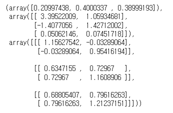
- 이 클래스는 EM알고리즘 사용(K-평균 알고리즘과 비슷)
- 클러스터 파라미터를 랜덤하게 초기화하고 수렴할 때까지 두 단계를 반복
- 샘플을 클러스터에 할당(기댓값 단계 - Expectation)
- 클러스터를 업데이트(최대화 단계 - maximization)
- K-평균과 차이점은 하드 클러스터가 아닌 소프트 클러스터 사용
- 기댓값 단계에서 알고리즘은 각 클러스터에 속할 확률을 예측
- 최대화 단계에서 각 클러스터가 데이터셋에 있는 모든 샘플을 사용해 업데이트
- 클러스터에 속할 추정 확률로 샘플에 가중치 적용, 이 확률을 샘플에 대한 클러스터의 책임이라고 지칭
- 최대화 단계에서 클러스터 업데이트는 책임이 가장 많은 샘플에 크게 영향을 받음
gm.converged_, gm.n_iter_(True, 6)
- 이 모델은 새로운 샘플을 가장 비슷한 클러스터에 손쉽게 할당(하드 군집) - predict()
- 특정 클러스터에 속할 확률에 예측할 수 있음(소프트 군집) - predict_proba()
gm.predict(X), gm.predict_proba(X)
- 가우시안 혼합 모델은 생성 모델
- 이 모델에서 새로운 샘플을 만들 수 있음
X_new, y_new = gm.sample(6)
X_new, y_new
- 주어진 위치에서 모델의 밀도 추정: score_samples()
- 샘플이 주어지면 이 메서드는 그 위치의 확률 밀도 함수의 로그 예측, 점수가 높을수로 밀도가 높음
gm.score_samples(X)
from matplotlib.colors import LogNorm

def plot_centroids(centroids, weights=None, circle_color='w', cross_color='k'):
    if weights is not None:
        centroids = centroids[weights > weights.max() / 10]
    plt.scatter(centroids[:, 0], centroids[:, 1],
                marker='o', s=35, linewidths=8,
                color=circle_color, zorder=10, alpha=0.9)
    plt.scatter(centroids[:, 0], centroids[:, 1],
                marker='x', s=2, linewidths=12,
                color=cross_color, zorder=11, alpha=1)

def plot_gaussian_mixture(clusterer, X, resolution=1000, show_ylabels=True):
    mins = X.min(axis=0) - 0.1
    maxs = X.max(axis=0) + 0.1
    xx, yy = np.meshgrid(np.linspace(mins[0], maxs[0], resolution),
                         np.linspace(mins[1], maxs[1], resolution))
    Z = -clusterer.score_samples(np.c_[xx.ravel(), yy.ravel()])
    Z = Z.reshape(xx.shape)

    plt.contourf(xx, yy, Z,
                 norm=LogNorm(vmin=1.0, vmax=30.0),
                 levels=np.logspace(0, 2, 12))
    plt.contour(xx, yy, Z,
                norm=LogNorm(vmin=1.0, vmax=30.0),
                levels=np.logspace(0, 2, 12),
                linewidths=1, colors='k')

    Z = clusterer.predict(np.c_[xx.ravel(), yy.ravel()])
    Z = Z.reshape(xx.shape)
    plt.contour(xx, yy, Z,
                linewidths=2, colors='r', linestyles='dashed')

    plt.plot(X[:, 0], X[:, 1], 'k.', markersize=2)
    plot_centroids(clusterer.means_, clusterer.weights_)

    plt.xlabel("$x_1$", fontsize=14)
    if show_ylabels:
        plt.ylabel("$x_2$", fontsize=14, rotation=0)
    else:
        plt.tick_params(labelleft=False)
plt.figure(figsize=(8, 4))
plot_gaussian_mixture(gm, X)
plt.show()
- 점수의 지숫값을 계산하면 샘플의 위치에서 PDF 값을 얻을 수 있음, 이 값은 하나의 확률 밀도 / 즉, 0에서 1까지 값이 아닌 어떤 양수값도 가능
- 샘플이 특정 지역 안에 속할 확률을 예측하려면 그 지역에 대해 PDF를 적분해야 함(가능한 샘플 위치 전 지역에 대해 적분해 더하면 1이 됨)
- 특성이나 클러스터가 많거나 샘플이 적을 때는 EM이 최적의 솔루션으로 수렴하기 어려움
- 어려움 해결을 위해 알고리즘이 학습할 파라미터의 개수를 제한
- 클러스터의 모양과 방향의 범위를 제한 -> 공분산 행렬에 제약을 추가
covariance_type 매개변수를 사용해 이 알고리즘이 찾을 공분산 행렬을 제한할 수 있습니다.
- "full"(기본값): 제약이 없습니다. 모든 클러스터가 어떤 크기의 타원도 될 수 있습니다.
- "tied": 모든 클러스터가 동일하지만 어떤 타원도 가능합니다(즉, 공분산 행렬을 공유합니다).
- "spherical": 모든 클러스터가 원형이지만 지름은 다를 수 있습니다(즉, 분산이 다릅니다).
- "diag": 클러스터는 어떤 크기의 타원도 될 수 있지만 타원은 축에 나란해야 합니다(즉, 공분산 행렬이 대각 행렬입니다).
gm_full = GaussianMixture(n_components=3, n_init=10, covariance_type="full", random_state=42)
gm_tied = GaussianMixture(n_components=3, n_init=10, covariance_type="tied", random_state=42)
gm_spherical = GaussianMixture(n_components=3, n_init=10, covariance_type="spherical", random_state=42)
gm_diag = GaussianMixture(n_components=3, n_init=10, covariance_type="diag", random_state=42)
gm_full.fit(X)
gm_tied.fit(X)
gm_spherical.fit(X)
gm_diag.fit(X)
def compare_gaussian_mixtures(gm1, gm2, X):
plt.figure(figsize=(9, 4))
plt.subplot(121)
plot_gaussian_mixture(gm1, X)
plt.title('covariance_type="{}"'.format(gm1.covariance_type), fontsize=14)
plt.subplot(122)
plot_gaussian_mixture(gm2, X, show_ylabels=False)
plt.title('covariance_type="{}"'.format(gm2.covariance_type), fontsize=14)
compare_gaussian_mixtures(gm_tied, gm_spherical, X)
plt.show()
2 - 1. 가우시안 혼합을 사용한 이상치 탐지
- 밀도가 낮은 지역에 있는 모든 샘플을 이상치로 볼 수 있음
- 사용할 밀도 임계값 설정
- 예로 제조 회사의 결함 제품 비율: 4%
- 밀도 임계값을 4%로 설정하면 밀도가 낮은 지역에 있는 샘플의 4%를 얻음
- 만약 거짓 양성(완벽한 정상이 결함으로 분류된다면)이 너무 많을 경우 임계값을 낮춤
- 반대로 거짓 음성이 너무 많으면(결함 제품이 결함으로 분류되지 않을 경우) 임계값을 더 높임
- 이는 일반적인 정밀도/재현율 트레이드 오프
from sklearn.utils.extmath import density
densities = gm.score_samples(X)
density_threshold = np.percentile(densities, 4)
anomalies = X[densities < density_threshold]

plt.figure(figsize=(8, 4))

plot_gaussian_mixture(gm, X)
plt.scatter(anomalies[:, 0], anomalies[:, 1], color='r', marker='*')
plt.ylim(top=5.1)

plt.show()
- 비슷한 작업은 특이치 탐지
- 이상치로 오염되지 않은 '깨끗한' 데이터셋에서 훈련한다는 것이 이상치 탐지와 다름
- 이상치 탐지는 데이터셋을 정제하는 데 자주 사용
- 가우시안 혼합 모델은 이상치를 포함해 모든 데이터에 맞추려고 합니다. 따라서 이상치가 너무 많으면 모델이 정상치를 바라보는 시각이 편향되고 일부 이상치를 정상으로 잘못 생각할 수 있습니다.
- 이런 일이 일어나면 먼저 한 모델을 훈련하고 가장 크게 벗어난 이상치를 제거합니다. 그다음 정제된 데이터셋에서 모델을 다시 훈련합니다.
- 또 다른 방법은 안정적인 공분산 추정 방법을 사용하는 것(EllipticEnvelope 클래스를 참고)
기능도 함수
from scipy.stats import norm

xx = np.linspace(-6, 4, 101)
ss = np.linspace(1, 2, 101)
XX, SS = np.meshgrid(xx, ss)
ZZ = 2 * norm.pdf(XX - 1.0, 0, SS) + norm.pdf(XX + 4.0, 0, SS)
ZZ = ZZ / ZZ.sum(axis=1)[:,np.newaxis] / (xx[1] - xx[0])

from matplotlib.patches import Polygon

plt.figure(figsize=(8, 4.5))

x_idx = 85
s_idx = 30

plt.subplot(221)
plt.contourf(XX, SS, ZZ, cmap="GnBu")
plt.plot([-6, 4], [ss[s_idx], ss[s_idx]], "k-", linewidth=2)
plt.plot([xx[x_idx], xx[x_idx]], [1, 2], "b-", linewidth=2)
plt.xlabel(r"$x$")
plt.ylabel(r"$\theta$", fontsize=14, rotation=0)
plt.title(r"Model $f(x; \theta)$", fontsize=14)

plt.subplot(222)
plt.plot(ss, ZZ[:, x_idx], "b-")
max_idx = np.argmax(ZZ[:, x_idx])
max_val = np.max(ZZ[:, x_idx])
plt.plot(ss[max_idx], max_val, "r.")
plt.plot([ss[max_idx], ss[max_idx]], [0, max_val], "r:")
plt.plot([0, ss[max_idx]], [max_val, max_val], "r:")
plt.text(1.01, max_val + 0.005, r"$\hat{L}$", fontsize=14)
plt.text(ss[max_idx]+ 0.01, 0.055, r"$\hat{\theta}$", fontsize=14)
plt.text(ss[max_idx]+ 0.01, max_val - 0.012, r"$Max$", fontsize=12)
plt.axis([1, 2, 0.05, 0.15])
plt.xlabel(r"$\theta$", fontsize=14)
plt.grid(True)
plt.text(1.99, 0.135, r"$=f(x=2.5; \theta)$", fontsize=14, ha="right")
plt.title(r"Likelihood function $\mathcal{L}(\theta|x=2.5)$", fontsize=14)

plt.subplot(223)
plt.plot(xx, ZZ[s_idx], "k-")
plt.axis([-6, 4, 0, 0.25])
plt.xlabel(r"$x$", fontsize=14)
plt.grid(True)
plt.title(r"PDF $f(x; \theta=1.3)$", fontsize=14)
verts = [(xx[41], 0)] + list(zip(xx[41:81], ZZ[s_idx, 41:81])) + [(xx[80], 0)]
poly = Polygon(verts, facecolor='0.9', edgecolor='0.5')
plt.gca().add_patch(poly)

plt.subplot(224)
plt.plot(ss, np.log(ZZ[:, x_idx]), "b-")
max_idx = np.argmax(np.log(ZZ[:, x_idx]))
max_val = np.max(np.log(ZZ[:, x_idx]))
plt.plot(ss[max_idx], max_val, "r.")
plt.plot([ss[max_idx], ss[max_idx]], [-5, max_val], "r:")
plt.plot([0, ss[max_idx]], [max_val, max_val], "r:")
plt.axis([1, 2, -2.4, -2])
plt.xlabel(r"$\theta$", fontsize=14)
plt.text(ss[max_idx]+ 0.01, max_val - 0.05, r"$Max$", fontsize=12)
plt.text(ss[max_idx]+ 0.01, -2.39, r"$\hat{\theta}$", fontsize=14)
plt.text(1.01, max_val + 0.02, r"$\log \, \hat{L}$", fontsize=14)
plt.grid(True)
plt.title(r"$\log \, \mathcal{L}(\theta|x=2.5)$", fontsize=14)

plt.show()
2 - 2. 클러스터 개수 선택하기
- K-평균에서는 이너셔, 실루엣 점수를 사용해 적절한 클러스터 개수를 선택
- 가우시안에서는 BIC, AIC와 같은 이론적 정보 기준을 최소화하는 모델 찾음
BIC=log(m)p−2log(L^)
AIC=2p−2log(L^)
- m은 샘플의 개수입니다.
- p는 모델이 학습할 파라미터 개수입니다.
- L^은 모델의 가능도 함수의 최댓값입니다. 이는 모델과 최적의 파라미터가 주어졌을 때 관측 데이터 X의 조건부 확률입니다.
- BIC, AIC는 모두 학습할 파라미터가 많은 모델에게 벌칙을 가하고 데이터에 잘 학습하는 모델에게 보상
- 둘의 선택은 대부분 동일하지만 다를 경우, BIC가 선택하한 모델이 AIC가 선택한 모델보다 간단한 파라미터가 적은 경향
- 대규모 데이터셋에서는 잘 안맞음
gm.bic(X), gm.aic(X)
gms_per_k = [GaussianMixture(n_components=k, n_init=10, random_state=42).fit(X)
             for k in range(1, 11)]

bics = [model.bic(X) for model in gms_per_k]
aics = [model.aic(X) for model in gms_per_k]

plt.figure(figsize=(8, 3))
plt.plot(range(1, 11), bics, "bo-", label="BIC")
plt.plot(range(1, 11), aics, "go--", label="AIC")
plt.xlabel("$k$", fontsize=14)
plt.ylabel("Information Criterion", fontsize=14)
plt.axis([1, 9.5, np.min(aics) - 50, np.max(aics) + 50])
plt.annotate('Minimum',
             xy=(3, bics[2]),
             xytext=(0.35, 0.6),
             textcoords='figure fraction',
             fontsize=14,
             arrowprops=dict(facecolor='black', shrink=0.1)
            )
plt.legend()

plt.show()
- K = 3에서 BIC, AIC 모두 가장 작음, 최선의 선택
2 - 3. 베이즈 가우시안 혼합 모델
- 최적의 클러스 개수를 수동으로 찾지 않고 불필요한 클러스터의 가중치를 0으로 만듦
- 클러스터 개수 n_components를 최적의 클러스터 개수보다 크다고 믿을 만한 값으로 지정
from sklearn.mixture import BayesianGaussianMixture
bgm = BayesianGaussianMixture(n_components = 10, n_init = 10)
bgm.fit(X)
np.round(bgm.weights_, 2)

plt.figure(figsize=(8, 5))
plot_gaussian_mixture(bgm, X)
plt.show()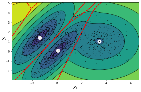
- 알고리즘이 자동으로 3개의 클러스터가 필요하다는 것을 감지
- 베타 분포: 고정 범위 안에 놓인 값을 가진 확률 변수를 모델링할 떄 자주 사용, 범위는 0 ~ 1

bgm_low = BayesianGaussianMixture(n_components=10, max_iter=1000, n_init=1,
                                  weight_concentration_prior=0.01, random_state=42)
bgm_high = BayesianGaussianMixture(n_components=10, max_iter=1000, n_init=1,
                                  weight_concentration_prior=10000, random_state=42)
nn = 73
bgm_low.fit(X[:nn])
bgm_high.fit(X[:nn])
np.round(bgm_low.weights_, 2)
np.round(bgm_high.weights_, 2)

- 다른 농도 값으로 동일한 데이터에서 다른 개수의 클러스터 생성
plt.figure(figsize=(9, 4))

plt.subplot(121)
plot_gaussian_mixture(bgm_low, X[:nn])
plt.title("weight_concentration_prior = 0.01", fontsize=14)

plt.subplot(122)
plot_gaussian_mixture(bgm_high, X[:nn], show_ylabels=False)
plt.title("weight_concentration_prior = 10000", fontsize=14)

plt.show()
from sklearn.datasets import make_moons
X_moons, y_moons = make_moons(n_samples=1000, noise=0.05, random_state=42)

bgm = BayesianGaussianMixture(n_components=10, n_init=10, random_state=42)
bgm.fit(X_moons)

#타원형이 아닌 클러스터에 가우시안 혼합 모델을 사용

def plot_data(X):
    plt.plot(X[:, 0], X[:, 1], 'k.', markersize=2)

plt.figure(figsize=(9, 3.2))

plt.subplot(121)
plot_data(X_moons)
plt.xlabel("$x_1$", fontsize=14)
plt.ylabel("$x_2$", fontsize=14, rotation=0)

plt.subplot(122)
plot_gaussian_mixture(bgm, X_moons, show_ylabels=False)

plt.show()
2 - 4. 이상치 탐지와 특이치 탐지를 위한 다른 알고리즘
- PCA(그리고 inverse_transform() 메서드를 가진 다른 차원 축소 기법)
- 보통 샘플의 재구성 오차와 이상치의 재구성 오차를 비교하면 일반적으로 후자가 더 큼. 이는 종종 매우 효과적인 이상치 탐지 기법
- Fast-MCD
- EllipticEnvelope 클래스에서 구현된 알고리즘, 이상치 감지, 특히 데이터셋 정제할 때 사용
- 보통 샘플(정상치)가 혼합된 것이 아니라 하나의 가우시안 분포에서 생성되었다고 가정
- 가우시안 분포에서 생성되지 않은 이상치로 데이터셋이 오염되었다고 가정
- 알고리즘이 가우시안 분포의 파라미터를(정상치를 둘러싼 타원 도형을) 추정할 때 이상치로 의심되는 샘플을 무시, 이런 기법은 알고리즘이 타원형을 잘 추정하고 이상치를 잘 구분하도록 도움
- LOF(local outlier factor)
- 이상치 탐지에 탁월, 주어진 샘플 주위의 밀도와 이웃 주위의 밀도를 비교
- 이상치는 종종 k개의 최근접 이웃보다 격리
- one-class SVM
- 특이치 탐지에 탁월
- 원본 공간으로부터 고차원 공간에 있는 샘플을 분리, 원본 공간에서는 모든 샘플을 둘러싼 작은 영역을 찾는 것에서 해당
- 새로운 샘플이 이 영역 안에 놓이지 않는다면 이는 이상치(조정할 파라미터가 작음)
- 고차원 데이터셋에는 탁월하지만 SVM과 마찬가지로 대규모 데이터 셋으로 확장은 불가능
핸즈온 머신러닝 - 교보문고
사이킷런, 케라스, 텐서플로 2를 활용한 머신러닝, 딥러닝 완벽 실무 | 머신러닝 전문가로 이끄는 최고의 실전 지침서 텐서플로 2.0을 반영한 풀컬러 개정판 이 책의 원서는 출간 직후부터 미국
www.kyobobook.co.kr
728x90
반응형
LIST
'Machine Learning의 민족 > 핸즈온 머신러닝' 카테고리의 다른 글
| < 핸즈온 머신러닝 - 비지도 학습1 - 군집 > (0) | 2022.06.14 |
|---|---|
| < 핸즈온 머신러닝 - 차원 축소 > (0) | 2022.06.09 |
| < 핸즈온 머신러닝 - 앙상블 학습과 랜덤포레스트 > (0) | 2022.06.07 |
| < 핸즈온 머신러닝 - 결정 트리 > (0) | 2022.06.03 |
| < 핸즈온 머신러닝 - SVM > (0) | 2022.06.02 |
'Machine Learning의 민족/핸즈온 머신러닝' Related Articles
more


Comments